As we all know, risk is an important factor in making decisions. In many areas, decision makers must often choose a course of action in the face of risks. In order to monitor risks timely and minimize the loss caused by risk, it is necessary to analyze and compare a great variety of risks.

There exist many ways to depict and measure risk because every decision maker has its own perception of risk. Variance and standard deviation were the traditional risk measures and first applied in the selection of portfolios by Markowitz (1952). After about 40 years, value at risk (VaR) was introduced in financial risk management by Guldimann (1995). Now, it is adopted by many financial institutions to control the risk of loss. Unfortunately, value at risk does not possess subadditivity. Therefore, tail value at risk (TVaR) as a natural remedy for the shortcoming of VaR was proposed by Artzner et al. (1997). These risk measures have become important tools in the stochastic risk analysis fields. In the stochastic environment, risk usually was regarded as a random variable and there were many methods to rank the random variables. The applications of stochastic dominance can be found in welfare, poverty and inequality, such as Shaked and Shanthikumar (1994), Barrett and Donald (2003).

In fuzzy environment, many researchers regarded risk as a fuzzy variable and adopted fuzzy theory and methodology as an approach to risk analysis (Zmeskal, 2005; Lee and Chen, 2008). From the beginning of the development of fuzzy set theory (Zadeh, 1965), the problem of fuzzy variable dominance was studied. Lee and Li (1988) proposed comparison of fuzzy numbers based on the probability measure of fuzzy events. Tran and Duckstein (2002) compared fuzzy numbers using a fuzzy distance measure. Nojavan and Ghazanfari (2006) presented fuzzy ranking method by desirability index. Peng et al. (2005) and Peng et al. (2007) provided a fuzzy dominance method based on credibility measure. Recently, Peng (2008) presented the concept of credibilistic VaR via credibility theory to measure fuzzy risk. Afterward, Peng (2009b) proposed average value at risk (AVaR) in fuzzy risk analysis. These methods have played important roles in fuzzy risk analysis problems.

However, many surveys showed that some imprecise phenomena behave neither like randomness nor like fuzziness. In order to deal with this uncertainty different from randomness and fuzziness, Liu (2007) founded uncertainty theory based on normality, self-duality, coun-table subadditivity, and product measure axioms in 2007, and it was refined by Liu (2010a). As a new tool to study the uncertainty in human systems, uncertainty theory motivates a new area of risk analysis called uncertain risk analysis. Here the risk is defined as the accidental loss plus uncertain measure of such loss (Liu, 2010b). The fact that risk is usually not a known constant shows that it is reasonable to represent risk by uncertain variable. Up to now, many significant risk measures have been proposed from different angles in uncertain risk analysis. Peng (2009a) suggested the VaR and TVaR based on uncertainty theory. Liu (2010b) provided the risk index to measure some risk loss. Peng and Li (2010, 2011) studied the distortion risk measure and spectral measure of uncertain risk, respectively. These uncertain measures can be widely used as tools of risk analysis in uncertain environment. In this paper, we aim to define some comparison rules of risks within the framework of uncertainty theory and discuss the relationship between these comparison rules and uncertain risk measures. The risk comparison approach is different from those in stochastic and fuzzy environment. It is worthwhile to compare risks on the basis of these uncertain measures.

The remainder of this paper is organized as follows. Section 2 presents preliminaries in the uncertainty theory. The concepts of some risk measures based on the uncertainty theory are given in section 3. Section 4 introduces three types of comparison rules of risks. In section 5, we build the bridges between uncertain risk measures and comparison rules of risks. Section 6 gives some comparable illustrations. The last section contains some concluding remarks.

Let Γ be a nonempty set. A collection L of subsets of Γ is a σ -algebra. Uncertain measure M introduced by Liu (2007) is a set function if it satisfies the following axioms:

(1) (Normality) M { Γ } =1;

(2) (Self-duality) M{Λ} M{Λc} =1 for any Λ ∈ L ;

(3) (Subadditivity) For every countable sequence of events { Λ i }, we have

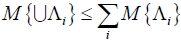
The triplet (Γ L, M) is called an uncertain space. In order to obtain an uncertain measure of compound event, Liu (2009) defined a product uncertain measure which produces the forth axiom of uncertainty theory:

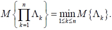
(4) (Product axiom) Let (Γ k, Lk, Mk) be uncertain space for k = 1, 2, … , n. Then the product uncertain measure M is an uncertain measure on the product σ - algebra Π Lk satisfying

An uncertain variable is defined as a measurable function from an uncertain space (Γ , L, M ) to the set of real numbers. The uncertainty distribution Φ : ？ → [0, 1] of an uncertain variable ξ is defined by Liu (2007) as

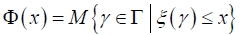
and the inverse function Φ^-1 is called the inverse uncertainty distribution of ξ .

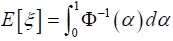
Expected value is the average value of uncertain variable in the sense of uncertain measure, and represents the size of uncertain variable. The expected value of uncertain variable ξ is defined by Liu (2007) as

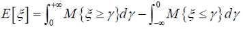
provided that at least one of the two integrals is finite. Liu (2010a) has proved that

if the expected value of uncertain variable ξ exists.

Let ξ be an uncertain variable with finite expected value E[ξ]. The variance of ξ is defined as V [ξ ] = E

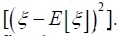
And the standard deviation of ξ is defined as

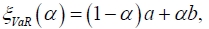
An uncertain variable ξ is called linear if it has a linear uncertainty distribution

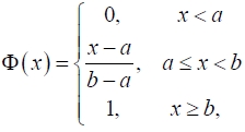
denoted by L(a, b) where a and b are real numbers with a < b, and the inverse uncertainty distribution is

Φ^-1 (α) = (1？α )a αb, 0 < α < 1.

The expected value and variance are (a + b)/2 and (b?a)²/12.

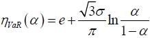
An uncertain variable ξ is called normal if it has a normal uncertainty distribution

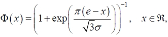
denoted by N (e, σ), where e and σ are real numbers with σ > 0, and the inverse uncertainty distribution is

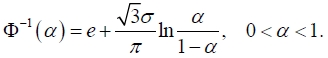
The expected value and variance are e and σ².

Risk measure is the core of risk analysis. Here we introduce some uncertain risk measures quoted from Peng (2009a, 2009b).

Definition 1: (Peng, 2009a) Let ξ be an uncertain variable and α ∈(0，1) be the risk confidence level. Then the function ξ_VaR : (0, 1) → ？ such that

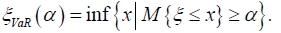
From this definition, we can see that ξ_VaR just is the generalized inverse function of Φ^-1 (α).

The VaR measures of linear uncertain variable ξ and normal uncertain variable η are

and

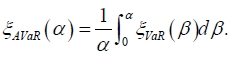
Definition 2: (Peng, 2009b) Let ξ be an uncertain variable and α ∈ (0，1) be the risk confidence level. Then the function ξ _AVaR : (0, 1) → ？ such that

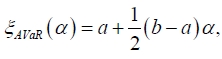
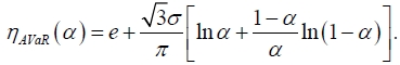
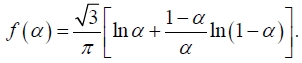
The AVaR measures of linear uncertain variable ξ and normal uncertain variable η are

and

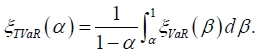
Definition 3: (Peng, 2009a) Let ξ be an uncertain variable and α ∈ (0，1) be the risk confidence level. Then the function ξ_TVaR : (0,1) → ？ such that

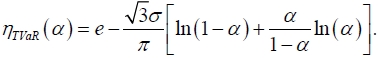
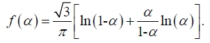
The TVaR measures of linear uncertain variable ξ and normal uncertain variable η are

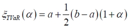
, and

A disadvantage of VaR is that it does not give the information about the severity of loss within and beyond the VaR level. Then, AVaR and TVaR mend this shortcoming. AVaR gives the estimation of loss within the VaR level and TVaR accounts for the severity of loss failure and not only the chance of failure. AVaR and TVaR are considered to provide the better measures of risk. Moreover, it can be verified that they all possess the properties of monotonicity, positive homogeneity, translation invariance, independence additivity.

Let ξ and η be two risks treated as uncertain variables with distribution functions Φ (x) and Ψ (x), respectively. This section will describe three types of rules to compare risks.

Definition 4: (First comparison rule) Let ξ and η be two risks with distribution functions Φ ( x) and Ψ ( x), respectively. ξis said to be smaller than η in first-order, if and only if Φ(x) ≤ Ψ(x) for all x∈？ , written

First comparison rule shows the possibility of same loss is small if the distribution function of risk always lies to the lower-right of the other. We can verify that the first comparison rule is reflexive, transitive and antisymmetric. That is, this rule is a partial order. Consequently, it is essential to introduce more applicable rules.

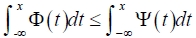
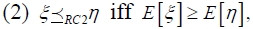
Definition 5: (Second comparison rule) Let ξ and η be two risks with distribution functions Φ ( x ) and Ψ ( x ), respectively. ξ is said to be smaller than η in secondorder, if and only if

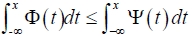
for all x∈？ , written

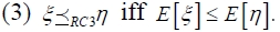
Definition 6: (Third comparison rule) Let ξ and η be two risks with distribution functions Φ( x ) and Ψ(x), respectively. ξ is said to be smaller than η in thirdorder, if and only if

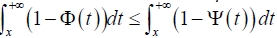
for all x？ , written

It is clear that the second and third comparison rules also meet reflexivity and transitivity. In addition,

implies both

and

In this section, we will investigate the relationships between uncertain measures and risk comparison rules.

Theorem 1: Let ξ and η be two risks with continuous distribution functions Φ( x) and Ψ(x), respectively. Then

iff ξ_VaR (α) ≥ η_VaR (α) for all α ∈(0, 1)

Proof: Necessity: If

i.e., Φ( x) ≤ Ψ(x) for all x∈?, we have inf

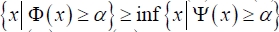
for all α , which means ξ VaR (α) ≥ ηVaR (α)

Sufficiency: For any x∈?, there is α ∈(0, 1) such that ξ _VaR (α) = x. ξ_VaR (α) ≥ η_VaR (α) shows Φ(x) = α ≤ Ψ(x).

Theorem 2: Let ξ and η be two risks with continuous distribution functions Φ(x) and Ψ(x), respectively. Then

iff ξ_VaR (α) ≥ η_VaR (α) for all α ∈(0, 1)

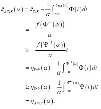
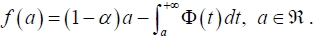
Proof: Necessity: Assuming that

and α ∈(0, 1) , we construct the function

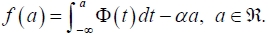
Next, we will prove that f(a) takes the minimum value at a = Φ^-1 (α) = ξ_VaR (α). On one hand, the inequality

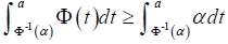
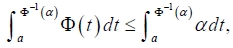
always holds for a ≥ Φ^-1 (α ) . Then,

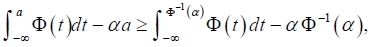
i.e.,

f (a) ≥ f (Φ^-1 (α )).

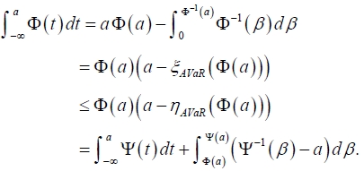
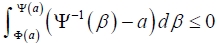
On the other hand, for a ≤ Φ ^?1 (α ), we have

i.e.,

That is to say, f (a) ≥ f (Φ^-1 (α )) for any a∈?. Then we have

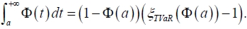
Sufficiency: Assume that ξ_VaR (α) ≥ η _VaR (α) for all α ∈ (0, 1). For a such that 0 < Φ(a) < 1, we have

By the α ≤ Ψ(a) ⇔ a ≥ Ψ ^-1 (α ) , it is obvious that

which implies

for a such that 0 < Φ(a) < 1. It is easy to verify this inequality holds when Φ(a) = 0 and Φ( a) =1. Hence ,

is proved.

Theorem 3: Let ξ and η be two risks with continuous distribution functions Φ( x) and Ψ(x), respectively. Then

iff ξ_VaR (α) ≤ η_VaR (α) for all α ∈( 0, 1).

Proof: Similarly, the necessity can be proved by constructing the function

And, we may prove the sufficiency after noticing

In the uncertainty theory, many types of uncertain variables can be used to describe risks. In this section, we concentrate on the comparison of risks with linear and normal uncertain distributions. First, according to the three risk comparison rules, we can obtain the following results for two risks with linear uncertain distributions.

Theorem 4: Let ξ ~ L (a₁, b₁) and η ~ L (a₂, b₂) be two risks with. b₁ ? a₁ < b₂ ? a₂ Then

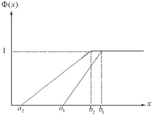
Proof: (1) It directly follows from the uncertain distribution of linear uncertain variable and definition of the first comparison rule. The result can be described in Figure 1.

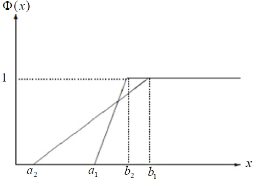
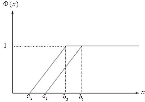
(2) It follows from the second comparison rule and Theorem 2 that

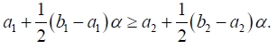
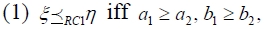
Under the hypothesis b₁ ？ a₁ < b₂ ? a₂ we get

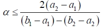
which yields b₁ + a₁ ≥ b₂ + a₂ i.e., E[ξ ] ≥ E[η ] . Then the result can be described in Figure 2 when b₁ < b₂ and Figure 3 when b₂ < b₁ .

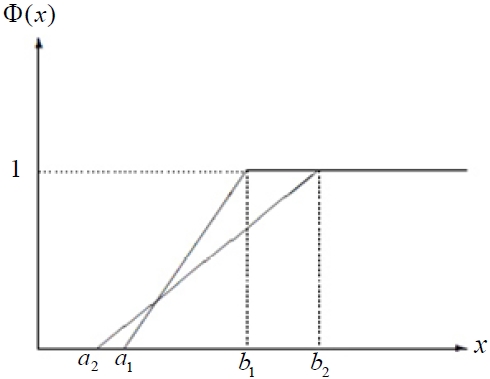
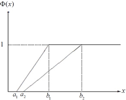
(3) By the analysis similar to (2), we have that

if and only if E[ξ ] ≤ E[η ] . We can describe the result in Figure 4 when a₁ < a₂ and Figure 5 when a₂ < a₁ .

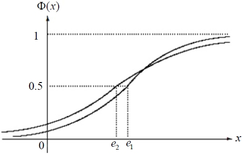
Next, we give the comparison results for two risks with normal uncertain distributions.

Theorem 5: Let ξ ~ N (e₁, σ₁ ) and η ~ N (e₂, σ₂ ). Then

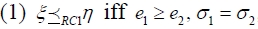
Proof: (1) It follows from the first comparison rule that

if and only if Φ( x) ≤ Ψ(x) for all x∈? i. e.,

for any x∈? and which shows e₁ ≥ e₂ and σ ₁ = σ ₂.

We know that the variance of an uncertain variable provides measure of the spread of the distribution around its expected value. So σ₁ = σ₂ implies the same spread of the distributions around theirs respective expected values. The result can be described in Figure 6.

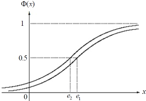
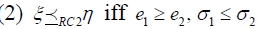
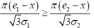
(2) It follows from the second comparison rule and Theorem 2 that for α ∈ (0, 1), f(α)(σ₂ ? σ₁) ≤ (e₁ ? e₂) where

So, we can obtain that

iff e₁ ≥ e₂ and σ₁ ≤ σ₂. In addition, σ₁ ≤ σ₂ indicates that the distribution of risk ξ is more tightly concentrated around its expected value. The result can be described in Figure 7.

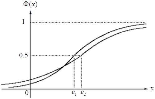
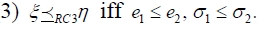
(3) It follows from the third comparison rule and Theorem 3 that for α ∈ (0, 1), f(α)(σ₂ ? σ₁) ≤ (e₂ ? e₁) where

So, we can obtain the result which can be described in Figure 8.

This paper has proposed a new approach to risk comparison by means of uncertain measures. We introduced the concepts of some uncertain measures and risk comparison rules within the framework of uncertain theory. Special attention is paid to building the bridges between uncertain measures and risk comparison rules. We described the three risk comparison rules by three kinds of uncertain measures: uncertain VaR, uncertain AVaR, and uncertain TVaR, respectively. Moreover, the results are applied in the risks with linear and normal uncertain distributions. This method will be a very helpful tool for studying risks whose characteristic is neither relative to randomness nor fuzziness. It should be emphasized that there are many ways to rank risks according to different uncertain measures. In risk analysis, choosing and finding a suitable risk measure to compare the risks will be constant exploration.