Continued greenhouse gas emissions at or above current rates will cause further warming and induce many changes in the global climate system in the 21st century that will likely be larger than those observed during the 20th century. Even if the concentrations of all greenhouse gases and aerosols is kept constant at the year 2000 levels, a further warming of about 0.1℃ per decade is expected. Temperature projections increasingly depend on specific emissions scenarios (Kim 1998, Hughes 2000, Schneider 2001, Walther et al. 2002, IPCC 2007).
Most ecologists recognise two aspects of biodiversity that must be considered when trying to quantify biodiversity: species richness (the number of species in a community) and relative abundance or equitability (the evenness with which individuals are spread out among the species in a community) (Whittaker et al. 2001, Barnard and Thuiller 2008). Biodiversity is usually defined in terms of molecules, genes, species and ecosystems and corresponds to four fundamental and hierarchically related levels of biological organisation (Campbell 2003). Because of the major influence of climate on range shifts, extinctions, distribution and vegetation types from continental to regional scale, it is expected that climate change will alter biodiversity considerably (Ricklefs 1987, Malanson 1993, Hughes 2000, Hansen and Dale 2001, Hansen et al. 2001, Bakkenes et al. 2002, Walther et al. 2002, Thuiller et al. 2005, Thuiller 2007, Shin et al. 2009, Wang et al. 2009, Rocchini et al. 2010, Kim 2012). The level of anthropogenic stress on biodiversity is far greater than that imposed by natural global climatic changes occurring in the re-
environmencent evolutionary past, including temperature increases, shifts in climate zones, melting of snow and ice, sea level increases, droughts, floods, and other extreme weather events. Natural systems are vulnerable to such changes because of their limited adaptive capacity (Pimm and Gittleman 1992, Vitousek 1994, Pimm et al. 1995, Chapin et al. 2000, Warren et al. 2001, Ihm et al. 2007, Fonty et al. 2009).
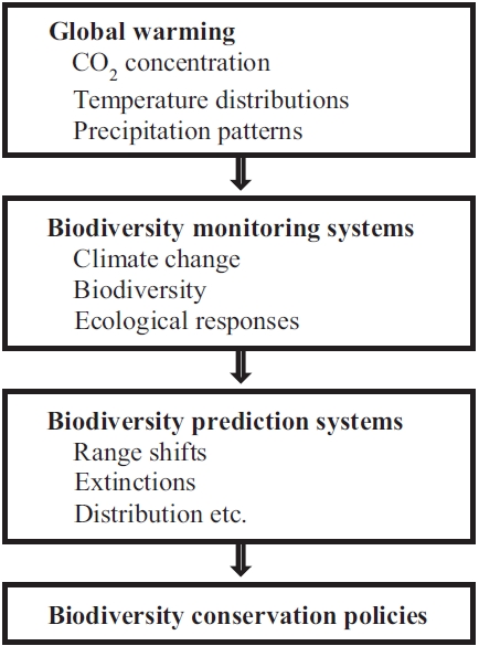
The objectives of this study are (a) to identify the impacts of global warming on biodiversity and (b) to provide explanations for predictive models and future changes in biodiversity (Fig. 1). These predictions need to be temporally and spatially explicit to allow ecologists and managers of protected areas to plan for the greatest number of species possible. The predictions based on credible modelling can guide the establishment of monitoring programmes to serve as early warning signs of the climate change trajectory. Furthermore, explicit predictions will allow safe limits of climate change to be defined and will aid in the development of policy guidelines on carbon emissions.
BIODIVERSITY PREDICTION MODELS
Allen et al. (2002) presented the species-energy hypothesis, which was intended to explain the latitudinal gradient of increasing species diversity from the poles to the equator. This model’s predictions are consistent with patterns of increasing numbers of plant and animal species with increasing mean air or water temperatures. Substantial evidence indicates that a broadly positive monotonic relationship between species richness and energy availability is common at geographical scales across temperate to polar areas (Dobzhansky 1950, Pianka 1966, Turner et al. 1988, Currie 1991, O'Brien 1998, Rutherford et al. 1999, Gaston 2000, Lennon et al. 2000, Francis and Currie 2003, Hawkins et al. 2003, Root et al. 2003, Hawkins and Pausas 2004, Evans et al. 2005, De Boeck et al. 2007, Ihm et al. 2007, Pe?uelas et al. 2007, Whittaker et al. 2007). The best correlates for terrestrial and marine animals are measures of energy, such as temperature, whereas the best correlates for plants tend to be measures of both water and energy, such as precipitation, temperature and net primary production (NPP) (Stevens 1989, Willig and Lyons 1998, Gaston 2000, Allen et al. 2002, Field et al. 2005, Mutke and Barthlott 2005, Barthlott et al. 2007, Kreft and Jetz 2007). The species richness of trees in East Asia, temperate Europe, and eastern North America increases with primary productivity. In contrast, factors such as mean annual precipitation, actual evapotranspiration or the number of days per year with rainfall have a much a closer relationship with species richness in the thermally more suitable tropics (Hawkins et al. 2003, Currie et al. 2004, Field et al. 2005, Mutke and Barthlott 2005, Barthlott et al. 2007, Kreft and Jetz 2007). The still developing "metabolic theory of ecology" (MTE) claims to derive ecological relationships from the structure of resource distribution networks, which is assumed to determine the scaling of metabolism with body mass from the effect of temperature on the rate of biological processes and from a range of macroecological patterns including diversity gradients (Allen et al. 2002, Brown et al. 2004, van der Meer 2006, Allen and Gillooly 2007). The observed diversity gradients are consistent with the MTE predictions across a wide range of taxonomic groups in almost all regions of the world (Hawkins et al. 2007). It is obvious that water is essential for any terrestrial system diversity at all, and it is possible that in systems where water is not limiting, enzyme kinetics could explain the observed gradients. Smaller scale gradients, such as those along mountain slopes, might also conform better to MTE predictions. It is anticipated that future climatic warming will change the distribution limits of many vascular plant species (Sætersdal et al. 1998). Stevens (1989) proposed Rapoport's rule as a possible explanation for the higher species richness of animals and plants in the tropics. The rule postulates that tropical species have smaller ranges on average, than temperate taxa because of the tolerance of temperate species to a broader range of environmental conditions. Rapoport's rule has been shown to apply to some groups in some continents, but the exceptions to the rule are numerous; therefore, its generalisability has been seriously questioned. Other perspectives for studying latitudinal gradients of species richness came from the mid-domain models developed during the 1990s (Colwell and Hurtt 1994, Willig and Lyons 1998, Colwell and Lees 2000, Arita 2005). In two-dimensional models, a similar peak in species richness appears in the centre of a bounded domain defined by latitude and longitude. The term "mid-domain models" comes from these predicted patterns of the highest richness at the middle of the gradient.
An increase in animal or plant species richness correlates with NPP or the Normalised Difference Vegetation Index (NDVI) (Alward et al. 1999, Evans et al. 2005, Leyequien et al. 2007, Woodward and Kelly 2008, Kim and You 2010) through a number of potential mechanisms, such as complementarity of resource use and positive interspecific interactions. This implies that an increase in the availability of resources favours an increase in diversity capacity (Morin 2000). At the global scale of investigation, NPP is a measure of resource availability for plants and is determined by geographic variations in climatic and edaphic characteristics and can be readily simulated. Woodward and Kelly (2008) investigated the premise that plant diversity is determined by NPP, while becoming aware that different geographical locations may have very different geological histories and species pools, which could lead to different NPP-diversity relationships. This model has two fundamental flaws concerning the species-energy hypothesis (Huston 2003, Brown et al. 2004). 1) Mean temperature does not correspond to the energy actually available to organisms, which is the energy stored in carbon compounds produced by photosynthesis. Although it is true that the tropics tend to be warmer than the temperate zone, higher temperatures do not necessarily result in higher plant productivity. 2) High species diversity occurs in cold or low-productivity environments.
The well-known species-area relationship (S = cAz) explains species richness on a local to regional scale (Whittaker et al. 2001, Thomas et al. 2004, Woodward and Kelly 2008, Ulrich and Fiera 2009, Henry et al. 2010). Area per se is a relatively weak predictor of species richness and explains only 6.6% of the global variation in plant species richness (Kreft and Jetz 2007). However, the explanatory power of area dramatically increases when spatial autocorrelation is explicitly modelled (57.4% deviance). This indicates strong neighbourhood effects.
Habitat factors (e.g., topography, soil, land use, disturbance, and climate), historical/evolutionary factors, and biotic factors (e.g., invasion, competition, predation, niche difference, and natural enemies) influence habitat and species differentiation of communities and might explain the higher biodiversity of geodiverse regions (Grime 1974, Connell 1978, Shmida and Wilson 1985, Rohde 1992, Palmer 1994, Pimm et al. 1995, Chapin et al. 2000, Sala et al. 2000, Whittaker et al. 2001, Hawkins et al. 2003, Currie et al. 2004, Hubbell 2005, 2006, Barthlott et al. 2007).
FUTURE CHANGES IN BIODIVERSITY
Table 1 includes response variables, model types, extents, explanatory variables and climate data or global climate models (GCMs) simulated, but most of the explanatory variables represent measures of water (precipitation, moisture availability index and water deficit), energy (temperature, NPP, and NDVI), ecophysiological responses, topographic complexity and population dynamics (Jetz and Rahbek 2002, Midgley et al. 2002, Hawkins et al. 2003, Venevsky and Veneskaia 2003, Lemoine et al. 2007). Furthermore, water variables tend to be the best predictors when the geographic scope of the data is restricted to tropical and subtropical areas, whereas water-energy variables dominate when colder areas are included. In cold regions, where energy inputs are lower and thus more likely to be limiting, energy interacts with water to explain richness gradients.
Although evidence for extinctions caused primarily by climate change is relatively limited, many projections suggest serious future concerns for many species (Thomas et al. 2004, Thuiller et al., 2005, Huntley et al. 2008, Olofsson et al. 2008, Sinervo et al. 2010). One estimate indicates that ~86% of the plant and animal species assessed are likely to be at increasingly high risk of extinction caused by climate change in the 21st century. At the local scale, Guisan and Theurillat (2000) and Dirnb?ck et al. (2003) showed that mountainous plants at high elevations are particularly susceptible to extinction. Up to 25% of the plant species now present in southern Europe may disappear by 2100 (Bakkenes et al. 2006).
Temperature is a better predictor of avian species richness than is NDVI in models restricted to a single measure of energy availability, but it is important to note that temperature and NDVI are correlated (Table 1) (Evans et al. 2005). NDVI measures are retained in most of the best-fitting spatial regression models. The relationship between avian communities and climatic conditions is dependent on the energy metric used, with species richness being more closely correlated with temperature than with the NDVI, which is a strong correlate of NPP (Evans et al. 2005, Leyequien et al. 2007).
Lemoine et al. (2007) developed spatial regression models and quantified the relationship between the pro-
[Table 1.] Biodiversity prediction models based on several methods
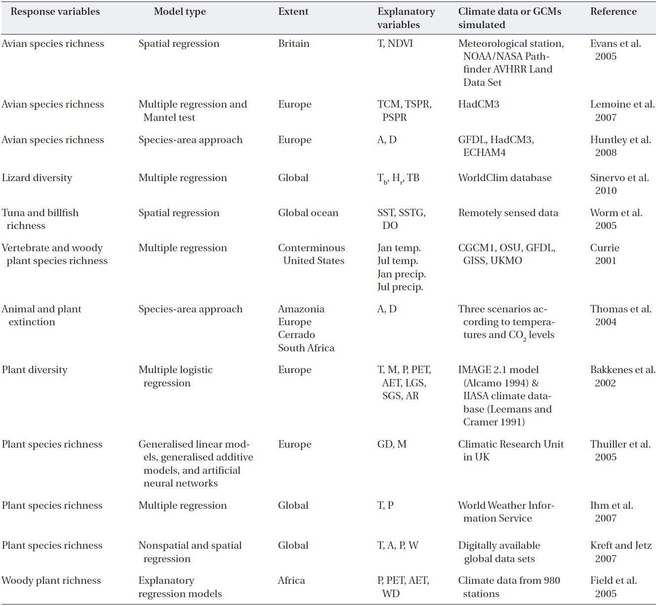
Biodiversity prediction models based on several methods
portion of migratory and resident bird species and climatic conditions (Table 1). They used the mean temperature of the coldest month (TCM), the mean spring temperature (TSPR, average of April, May and June) and spring precipitation (PSPR, average of April, May and June) as measures of climatic conditions in winter and during the breeding period. The spatial relationship between avian communities and climatic conditions was derived from spatial regression models in Europe (Lemoine and Bohning- Gaese 2003). The proportion of long- and short-distance migratory species was well described by TCM, TSPR and PSPR (
For six climate scenarios between 2070 and 2099, changes were estimated for 431 European breeding avian species using models relating species’ distributions in Europe to climate (Table 1) (Huntley et al. 2008). It was estimated that the average number of species breeding per 50-km grid square would decrease by 6.8-23.2%. The simulated reduction in mean range extent resulted in a reduction in the simulated mean number of breeding species per grid cell and hence a general decrease in local avian species richness across Europe. Of the scenarios examined, the smallest effect (a 6.8% average reduction in the number of species breeding in a 50-km grid square) was observed for the GFDL B2 scenario when assuming perfect dispersal, whereas the largest effect (a 56.4% average reduction in the number of species breeding in a 50-km grid square) was observed for the ECHAM4 A2 scenario when assuming dispersal failure (Ibanez et al. 2006).
The lizard diversity model, based on body temperature (Tb), hours of activity during reproduction (hr) and timing of breeding, assesses salient adaptations that affect thermal extinctions (Sinervo et al. 2010). Geo-referenced Tb samples indicate that local extinctions in 2009 averaged 4% worldwide. Global averages will increase four-fold to 16% by 2050 and nearly eight-fold to 30% by 2080, whereas equatorial extinctions will reach 23% by 2050 and 40% by 2080.
The richness of tuna and billfish species showed a consistent global pattern, indicating peaks of diversity at intermediate latitudes (15 to 30°N or S) and lower diversity toward the poles and at the equator (Table 1) (Worm et al. 2005). In an effort to determine which oceanographic variables might explain global patterns of predator diversity, they explored the effects of remotely sensed sea surface temperatures (SST) (mean and spatial gradients), dissolved oxygen levels, eddy kinetic energy, chlorophyll
For trees and birds, the positive coefficient on the linear term for July temperature indicates that richness initially increased with increasing temperature, but that the relationship decelerated (Table 1) (Currie 2001). Eventually, richness reached a maximum and then began to decrease. Multiple regression models including temperature and precipitation account statistically for 83-94% of the contemporary North American variation in species richness in trees and birds. Climate change should lead to variable changes in species richness across the contiguous United States. The results suggest that marked increases in the richness of most taxa are likely to occur in cool regions, whereas decreases in homoeotherm richness are likely to occur in parts of the South.
Thomas et al. (2004) explored methods for estimating animal and plant extinction based on the species-area relationship (S = cAz, where S is the number of species, A is the area, and c and z are constants). This relationship adequately predicts the numbers of animal and plant species that become extinct or threatened when the area available to them is reduced by climate change (Ib??ez et al. 2006, Huntley et al. 2008). Minimum expected climatechange scenarios for 2050 produce fewer projected "committed extinctions (18%) than do mid-range projections (24%) and about half of those predicted under maximum expected climate change (35%).
Bakkenes et al. (2002) studied a geographically explicit quantification of the possible effects of forecasted climate change on the diversity of the European flora (Table 1). A species-based probabilistic model, Euromove, has been developed. Euromove calculations resulted in climate envelopes for nearly 1,400 plant species. Euromove integrates calculated regression equations to analyse the effects of climate change on the European flora. According to Euromove calculations, the results show major changes for biodiversity by 2050. On average, 32% of the 1,990 species would disappear from each grid cell.
The relationship between the modelled percentage of species loss and the anomalies for the two most significantly correlated bioclimatic variables-growing-degree days (accumulated warmth) and the moisture availability index-was used to identify the potential causes of variation in predicted plant diversity changes across regions within and across scenarios (Thuiller et al. 2005) (Table 1). Multiple linear regression with the use of these two predictors explained 60% of the variance across scenarios. Applying the International Union for Conservation of Nature and Natural Resources (IUCN) Red List criteria to their projections showed that many European plant species could become severely threatened. More than half of the species they studied could be vulnerable or threatened by 2080. Expected species loss per pixel (a 50 × 50- km grid) proved to be highly variable across scenarios (27- 42%, averaged over Europe) and across regions (2.5-86%, averaged over scenarios).
Ihm et al. (2007) analysed 40 climatological and two geographic variables for 90 countries in the Northern Hemisphere to investigate the predictors that explained the variances in species richness (Table 1). When multiple regression models were used to evaluate this variance, the model
Kreft and Jetz (2007) used both non-spatial and spatial modelling techniques to test the predictive potential of variables. Predictive models of plant species diversity were developed globally by country to show that future plant diversity capacity has a strong dependence on changing climate (Table 1). A significant positive effect of average annual temperature on vascular plant species richness (8.5% deviance in the general linear model; GLM) was observed. Actual evapotranspiration emerged as the strongest single climatic predictor (28.6% deviance). Water- energy models that include interaction terms tend to have stronger explanatory power than do those with only main effects. They constructed a GLM and the spatial linear model (SLM) multi-predictor model (Kraft and Jetz 2007). The six explanatory variables included area (km2), potential evapotranspiration (mm/y), annual number of days with rainfall, number of 300-m elevation belts per geographic unit (range of elevation divided by 300) the number of different vegetation types and three-dimensional structural complexity. This model explained 65.9% of the observed deviance in a GLM framework and 70.2% in a spatial linear model.
A model that is grounded on biological relativity to water- energy dynamics is the interim general model (IGM1 and IGM2) of the climatic potential for woody plant richness (Field et al. 2005). IGM1 describes horizontal climate- richness relationships based on annual rainfall (Ran) and minimum monthly potential evapotranspiration (PETmin); IGM2 additionally incorporates vertical changes in climate due to topographic relief. For the southern subcontinent of Africa (from 15? S-35? S latitude), the re-described regression models apply to the full range of global variation in all independent climate variables in the woody plants of Kenya. They concluded that the IGMs are globally applicable and provide a fundamental baseline for systematically estimating differences in woody plant richness (Field et al. 2005). Predictions of actual woody plant richness using IGM2 are mostly reasonable or close fits, with a slight increase in precision found among IGM2 predictions.
The most obvious use of predictive variables and models is to predict species richness when actual values are unknown (Table 1) (Bakkenes et al. 2002, Field et al. 2005). First, the predictive models provide a line of evidence for evaluating whether or not this is the case elsewhere in the world. Second, given that they invoke dynamic climatological variables, the predictive models can be linked directly to GCMs and used to examine how future changes in climate could alter present-day richness patterns. Predictions at the macro scale can be incorporated as potential richness in analyses of how other variables relate to richness (O’Brien et al. 2000, Whittaker et al. 2001). The models of Kreft and Jetz (2007) successfully explain the species richness gradient, or the predicted global map confirms many regional trends and hotspots anticipated previously. They have shown that relatively few variables, namely a combination of high annual energy input with constant water supply and extraordinarily high spatiotopographic complexity, can accurately predict the future change in plant richness.
Many European endemic species will have little or no overlap between their present and potential future ranges (Huntley et al. 2008); such species face an enhanced extinction risk as a consequence of climatic change. Although many human activities exert pressures on wildlife, the magnitude of the potential effects estimated for European breeding birds emphasises the importance of climate change. The response of woody plant species to climate change in climate models can dramatically influence forecasts of potential future changes in avian diversity (Shanahan et al. 2001). Models assuming a strong time lag in the response of woody plants to climate change forecast significantly stronger decreases in avian species richness under climate change than do models in which woody plant species richness are allowed to show an instantaneous response to climate change. Future changes in the distribution of woody plants might be important for birds from a trophic perspective. Particularly in the tropics, many woody plants provide important food resources for avian consumers, including fleshy-fruited trees and shrubs for frugivorous species (Shanahan et al. 2001).
We suggest four strategies for researchers to monitor species distribution and reduce biodiversity loss by the negative impacts of climate change (Sala et al. 2000, Currie 2001, Hansen and Dale 2001, Bakkenes et al. 2002, Midgley et al. 2003, Thomas et al. 2004, Worm et al. 2005, Botkin et al. 2007, Kreft and Jetz 2007, Huntley et al. 2008). First, minimising greenhouse gas emissions and sequestering carbon to realise minimum expected climate warming could substantially reduce the loss in biodiversity. Second, conservation efforts need to be expanded in scale and scope to mitigate biodiversity loss, particularly on nature reserves. Third, mechanistic or empirical models could offer an alternative approach to forecasting the effects of climate change. We suggest that there is now a wide scope for an integrated framework to forecast the impacts of global change on biodiversity. Such a framework could integrate models for species persistence and consider multiple causes of biodiversity change. Fourth, biodiversity in many ecosystems is sensitive to global changes in the environment and land use, and realistic projections of biodiversity change will require an integrated effort by climatologists, ecologists, social scientists, and policy makers to improve future change scenarios. Refinement of these models will require quantitative regional analyses, and a study of the interactions between the factors to which local biodiversity is most sensitive.