In the linearly constrained adaptive array [1], the desired signal is estimated such that the array weights are updated iteratively by the linearly constrained least mean square (LMS) adaptive algorithm. It has been shown that the algorithm performs well if the desired signal and the interference signals are uncorrelated. It was shown that the signal interaction inherent in the algorithm causes partial cancellation of the desired signal in the array output even though the desired signal and the interference signals are uncorrelated [2]. If the interference signals are correlated with the desired signal, the signal interaction causes the desired signal to be partially or totally cancelled in the array output depending on the extent of correlation between the desired signal and the interference patterns.
To avoid the signal cancellation phenomenon, a variety of methods [2-9] have been proposed, such as a master-slave type array processor [2], a spatial smoothing approach [3], and an alternate mainbeam nulling method [4, 5].
In this paper, a novel approach to the general linearly constrained adaptive array [1] is presented to improve the nulling performance of the conventional linearly constrained adaptive arrays in coherent and noncoherent environments. The desired response is formed as the output of the conventional beamformer weighted by a gain factor. The input signals to the conventional beamformer are given by those to the adaptive array. The narrowband and broadband adaptive arrays are implemented with coherent and noncoherent interference patterns.
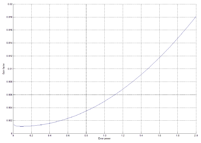
The nulling performance is shown to depend on the value of the gain factor such that there exists an optimal value of the gain factor that minimizes the error power between the array output and the desired signal.
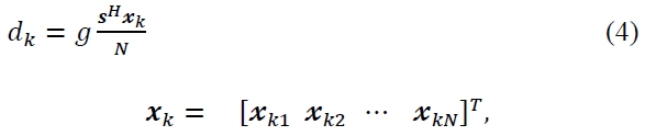
The proposed approach may be applied to the multipath environment in the area of wireless communications.
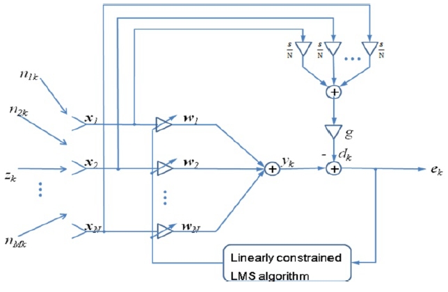
II. GENERAL LINEARLY CONSTRAINED NARROWBAND ADAPTIVE ARRAY
The general linearly constrained narrowband adaptive array with Q sensor elements is shown in Fig. 1. The weights ,
The optimization problem of finding an optimum weight vector for estimation of the desired signal is formulated as
where the weight vector
where β is the radian frequency of the desired signal,
The error signal is given by

where the

and the desired response
The iterative solution for the optimum weight vector may be found by the method of Lagrange multipliers [1], or what is called the general linearly constrained LMS algorithm,which is given by

Where
μ is convergence parameter, I is the N × N identity matrix,and * denotes complex conjugate.
The weight vector
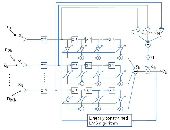
III. GENERAL LINEARLY CONSTRAINED BROADBAND ADAPTIVE ARRAY
A linearly constrained broadband adaptive array is shown to cancel out the desired signal in a coherent environment[2]. To prevent the signal cancellation phenomenon, a general linearly constrained broadband adaptive array is proposed. The general linearly constrained broadband adaptive array with N sensor elements followed by L taps per element is shown in Fig. 2.
The desired response
To minimize the mean square error output with a unit gain constrained in the look direction, the weights are adjusted iteratively by the general linearly constrained LMS algorithm [1] as follows.


where


It is worth noting that the constraint subspace is the orthogonal complement of the column space of
The array weights are updated such that the desired signal is estimated in a least mean square sense such that the array output power is minimized while maintaining the unit gain in the look direction.
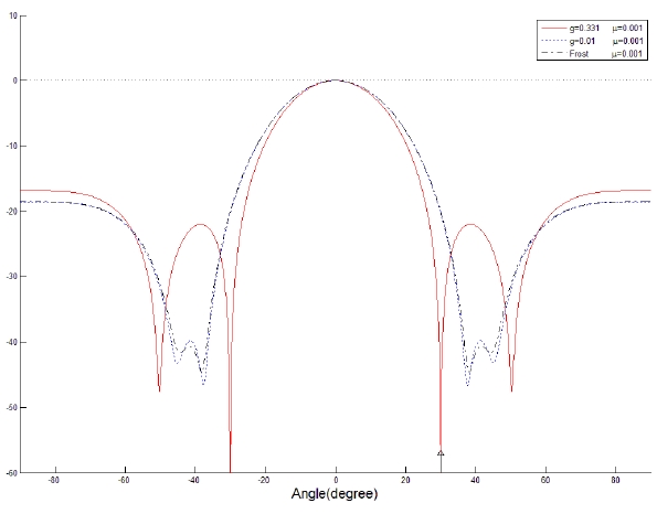
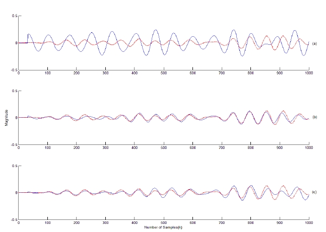
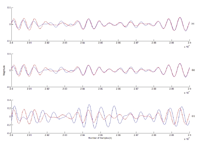
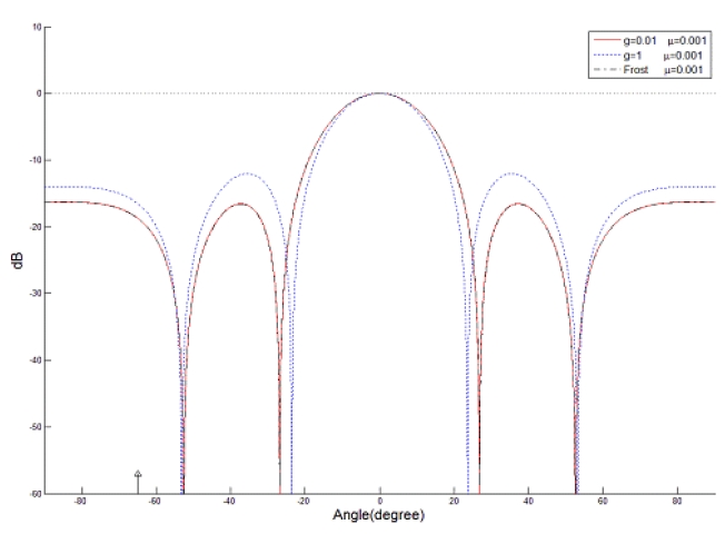
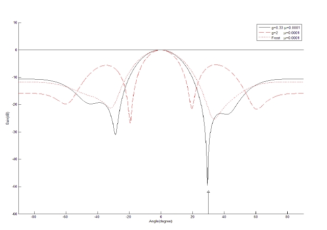
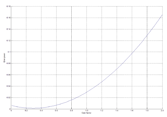
A narrowband linear array with 7 equispaced sensor elements is employed to examine the performance of the proposed method. The desired signal is assumed to be a sinusoid incident at the array normal. The cases for one and two coherent signal, and one noncoherent signal interference are simulated. The frequency of the noncoherent interferencen is assumed to be half that of the desired signal in the noncoherent case. The incoming signals are assumed to be plane waves. The nulling performances are compared with respect to the gain factor
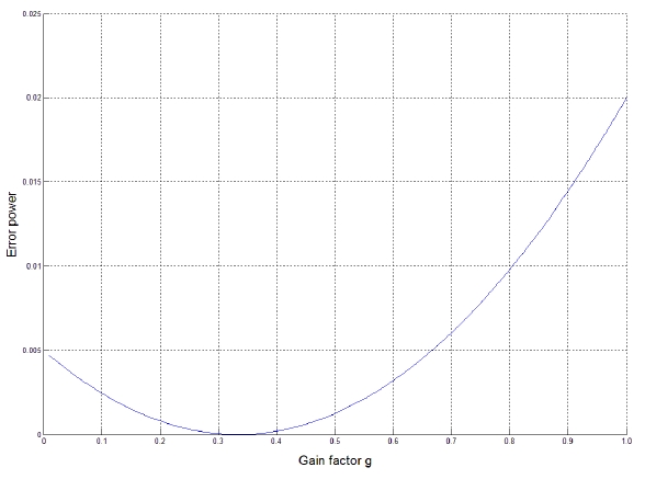
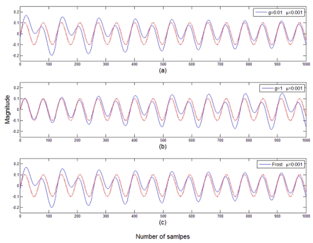
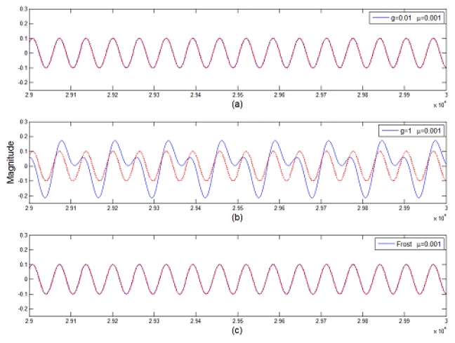
1) One Coherent Signal Interference Case
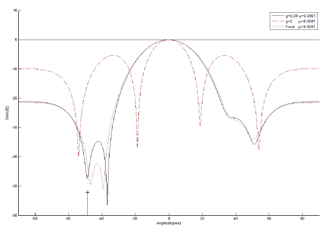
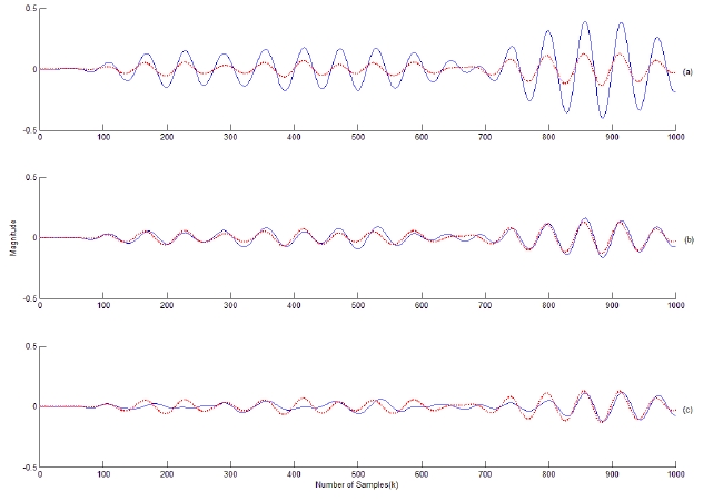
It is assumed that a coherent interference is incident at 30° from the array normal. The variation of the error power between the array output and the desired signal is displayed in terms of the gain factor
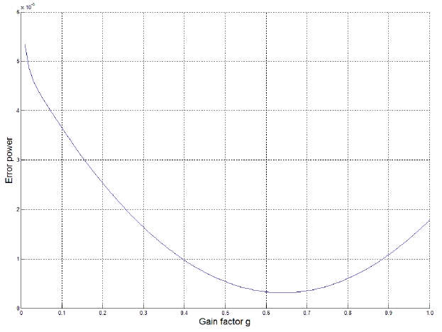
2) Two Coherent Signal Interference Case
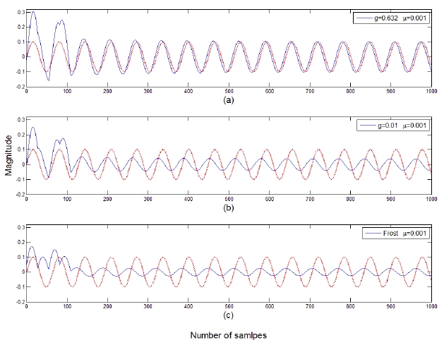
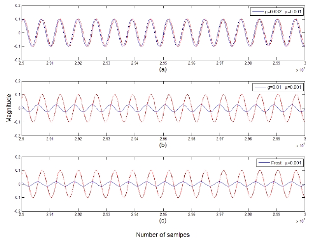
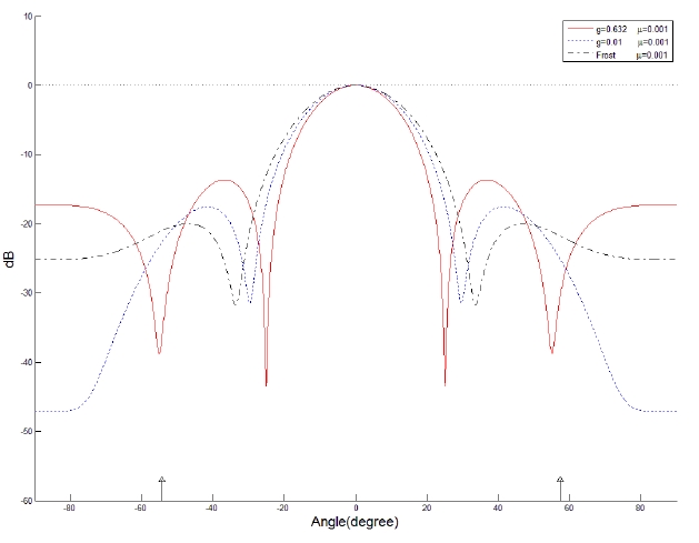
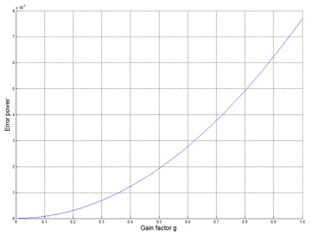
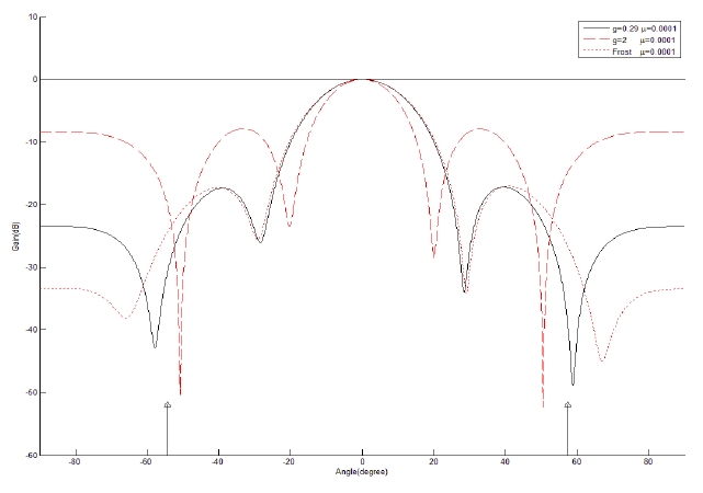
It is assumed that two coherent signal interferences are incident at -54.3° and 57.5° from the array normal. The variation in the error power between the array output and the desired signal is displayed in Fig. 7. The optimum value of
3) One Noncoherent Signal Interference Case
It is assummed that a noncoherent interference is incident at -64.9° from the array normal. The variation of the error power between the array output and the desired signal is displayed in Fig. 11. The optimum value of g is shown to be 0.0. The comparison of the array performance for
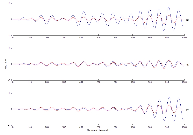
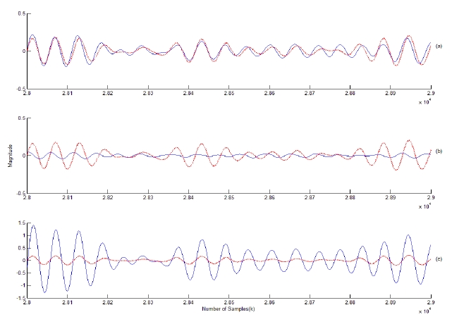
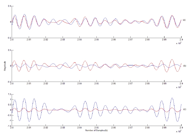
A broadband linear adaptive array with 5 sensor elements and 3 weights per element is simulated with incoming broadband signals. The broadband desired signal is generated by passing a white Gaussian random signal through a 4th-order Butterworth filter such that the bandwidth is 3 Hz with the upper and lower frequencies 8 Hz and 11 Hz, respectively. The incoming signals are assumed to be plane waves. The cases for one and two coherent signal and one noncoherent signal interferences are simulated. The sampling frequency is 608 Hz. The convergence parameter is assumed to be 0.0001.
1) One Coherent Interference Case
It is assummed that a coherent interference is incident at 30° from the array normal. The variation of the error power between the array output and the desired signal is displayed in Fig. 15. The optimum value of
2) Two Coherent Interference Case
It is assummed that two coherent signal interference patterns are incident at -54.3° and 57.5° from the array normal. The variation in the error power between the array output and the desired signal is displayed in Fig. 19.The optimum value of
3) One Noncoherent Interference Case
It is assumed that a noncoherent interference is incident at -48.5° from the array normal. The variation of the error power between the array output and the desired signal is displayed in Fig. 23. The optimum value of
A general linearly constrained adaptive array is proposed and implemented to examine its performance in coherent and noncoherent signal environments. The performance of the proposed approach is examined with narrowband and broadband adaptive arrays in different signal environments.
In the narrowband case, it is shown that the proposed approach performs best at an optimal gain factor in a coherent environment while it performs similarly to Frost’s array as the gain factor decreases in a noncoherent environment. In the broadband case, the proposed approach performs better at the optimal gain factor than does Frost’s array in a coherent environment while it yields a similar performance to Frost’s in a noncoherent environment.