As the cost of sensors and storage devices goes down rapidly, ubiquitous applications tend to capture and record a vast amount of data. As one example, digital memories that record everyday life have been an active area of research [Czerwinski et al. 2006; Lamming and Newman 1992]. Some healthcare applications monitor patients around the clock [Wilson and Atkeson 2004]. One key challenge in these systems is how to extract interesting or unusual information. When data is stored, it is hard to anticipate how the data will be searched in the future. Thus, providing appropriate indexes for data at the time when it is stored may not be feasible. Requiring users to annotate the data is inconvenient or even infeasible in certain cases.
In this paper, we propose an automatic way to detect unusual days (i.e., days with unusual mobility patterns) for individual users. In our detection system, we used the locations that a user visited during each day to build mobility profiles dynamically and to classify user days. For the evaluation, we used the location data of wireless users collected by wireless access points. Although we used wireless location data,which can be collected only where wireless connectivity was available, we expect that many pervasive devices (i.e., smart phones) are or will be equipped with a locationtracking mechanism such as global positioning system (GPS). Our system allows users to easily identify unusual days of their life, detect changes in their mobility patterns, and understand their mobility characteristics. These capabilities will benefit numerous pervasive systems that deal with a large amount of data.
Bush [1945] mentioned a forehead-mounted camera in his 1945 address; many realizations of such a camera are now available, including GoPro and Looxcie. Because these digital memories capture a large amount of data, it is hard to pinpoint interesting data. Numerous researchers have worked to address this challenge. However, to the best of our knowledge, we are the first in identifying unusual days by mobility data.
Another application domain that can benefit from our system is healthcare [Frost and Smith 2003; Wilson and Atkeson 2004]. Healthcare monitoring systems can continuously monitor patients. While some monitoring systems focus on generating warnings, others are used for long-term diagnostic purposes. Since it is likely to be inconvenient and inaccurate for patients to record their activities or behaviors, these systems automatically record patients’ activities through various sensors. These systems potentially record a large amount of data, and it thus becomes hard to retrieve or pinpoint important information. One way to apply our system is to use the user’s mobility patterns and extract significant changes in the patterns. These changes may help identify causes of changes in a patient’s medical conditions. For example, changes in sleeping patterns may indicate potential medical problems.
Our system may also help with mobility prediction [Song et al. 2006]. Predicting a user’s mobility is important support for pervasive applications (such as a mobile Voice over IP) and for some context-aware systems. Prediction systems often build a profile using the history of user mobility patterns. If a user’s mobility pattern changes significantly at a certain point in time, these predictors should dynamically adjust profiles. Our system can detect these changes, which can then be reported to the mobility predictors.
Section 2 describes wireless-network traces, and Section 3 presents our detection system. Section 4 presents the evaluation results of our system using wireless traces. Section 5 introduces a distillation application for digital memories that illustrates how our system can be used to decide an appropriate distillation level. Section 6 summarizes
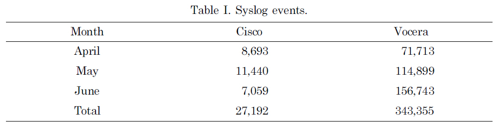
Syslog events.
[Table 2.] Number of user-days.
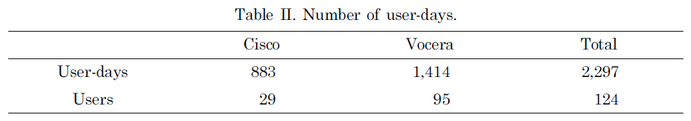
Number of user-days.
our finding and suggests future work.
We used traces collected at wireless access points (APs) on the Dartmouth College campus. These syslogtraces consisted of MAC addresses of wireless devices that were associated with each access point, collected at the granularity of seconds. Along with these traces, we used the geographical location of access points to consider the proximity among access points.
We used the traces collected during three full months: April, May, and June 2004 [Kotz et al. 2005]. Based on Dartmouth’s academic calendar, the months of April and May made up most of the spring term without any breaks. Spring term ended on June 8 and summer term did not start until June 24.
On the Dartmouth campus, there were two types of wireless network devices: onand-off and always-on devices. The former mostly consisted of laptops, and the latter consisted of Cisco Voice-Over-IP (VoIP) wireless mobile phones and Vocera devices, which were a smaller version of VoIP wireless phones with speech-recognition capability. In this study, we focused on the always-on devices to have a manageable sized data set: 27,192 events were generated by Cisco phones and 343,355 events were by Vocera phones. Table I shows the number of syslog events recorded for each month. However, our mobility analysis can also be used for the on-and-off devices without any modification.
Although a wireless network user can carry more than one device with multiple wireless network cards or can carry different devices from day to day, we assume that a MAC address represents one user of a wireless device. We define a
1The campus-wide syslog traces roll over at 4 AM every day.
In this section, we describe our mechanism for trace analysis. The goal of our approach was to identify days that were different from the user’s regular mobility pattern. For each day of the trace data, we computed the duration of stay at each location (e.g.,building) the user visited during that day. If this
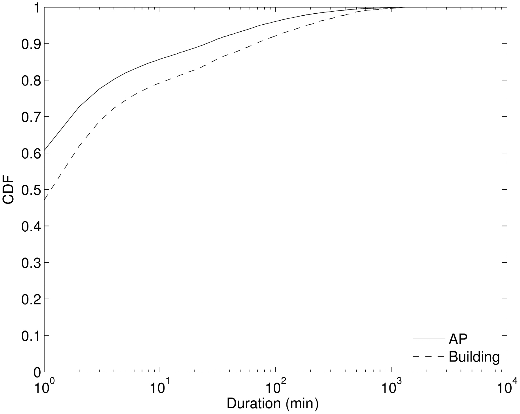
The density of APs on the Dartmouth College campus is high. The size of the campus is approximately 1 km2, and we observed 503 APs in the three-month traces under this study. Due to the high density, many of the APs were closely located and a wireless user visiting the same location may have associated with different APs during each visit. Even during one visit, a user’s device may have re-associated with multiple available APs in sequence. (This phenomenon is an instance of the ping-pong effect [Kim and Kotz 2007].) To discount these random events, we focused on the total duration of a user’s visits at each AP during each day, instead of the duration of each visit. We acknowledge that by using the total duration rather than a sequence of durations, we omitted some information. However, this was inevitable due to noise in the traces.
Figure 1 shows the cumulative distribution function (CDF) of the duration of stay across all daily durations for three months. The solid line shows durations at APs. For
the duration of APs, the 75th percentile is about 2-3 minutes. The percentage of short durations is high because a user associates with numerous APs while moving. Another reason is due to the ping-pong effect, which causes short-duration visits even when users are stationary; a device may associate with the closest AP for the most time, but briefly change to other nearby APs depending on the connectivity conditions
As mentioned earlier, our syslog trace lists APs that each user visited. At a given location, a user can be associated with one of many available APs, and may rapidly switch APs even while stationary due to changes in the radio environment. Thus, we believe that the set of APs that the user visited is too fine-grained to represent a user’s location history. Instead of using the actual set of APs, we aggregated APs into the buildings within which they were located. This aggregation effectively reduced the number of
3.3 Defining Regular Patterns Using Dynamic Profiling
After the aggregation steps, each user-day trace consists of a list of
In our approach, we did not use any extra knowledge. Instead, we dynamically updated a profile of each user. We used an exponentially-weighted moving average (EWMA) filter to update a user’s profile. The widely-used EWMA filter generates a moving average, while smoothing out noise. At time

where
Another interesting aspect of our approach is that we kept multiple profiles for each user. If a new user-day trace matched an existing profile, we updated the profile with the user-day trace. (We describe how we perform matching below.) If a new user-day trace did not match any of the existing profiles of that user, then we started a new profile. Each profile represented a class of that user’s mobility.
3.4 Detecting Unusual Patterns Using a Pearson’s Test
Given a user profile and a new user-day trace, we needed to decide whether or not the trace matched the profile. We considered several approaches. One popular test to decide whether two data sets were different was the t-Test. However, because this test compared the means between two distributions, it was not appropriate for our problem because our data consisted of paired sets, each data point consisting of a
The Pearson’s correlation test could be applied to our data set. To perform the Pearson’s test, two vectors under consideration need to be of the same length. Because we had 126 buildings, each user-day trace was converted to a vector of 126 elements with each element representing the duration at the particular building. Although this test assumes that the data follows a normal distribution, this assumption is not as strict as the data set becomes large. (Since our data set is large, we applied this test without checking whether or not our data in fact followed a normal distribution.) Given two variables
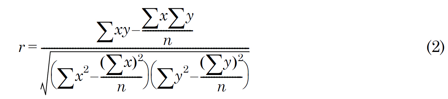
where
In this section, we present the results of our detection system using the Dartmouth wireless trace as the location data. We list mobility observations we made from this analysis, illustrate how our system classifies user-days, and summarize its capabilities.
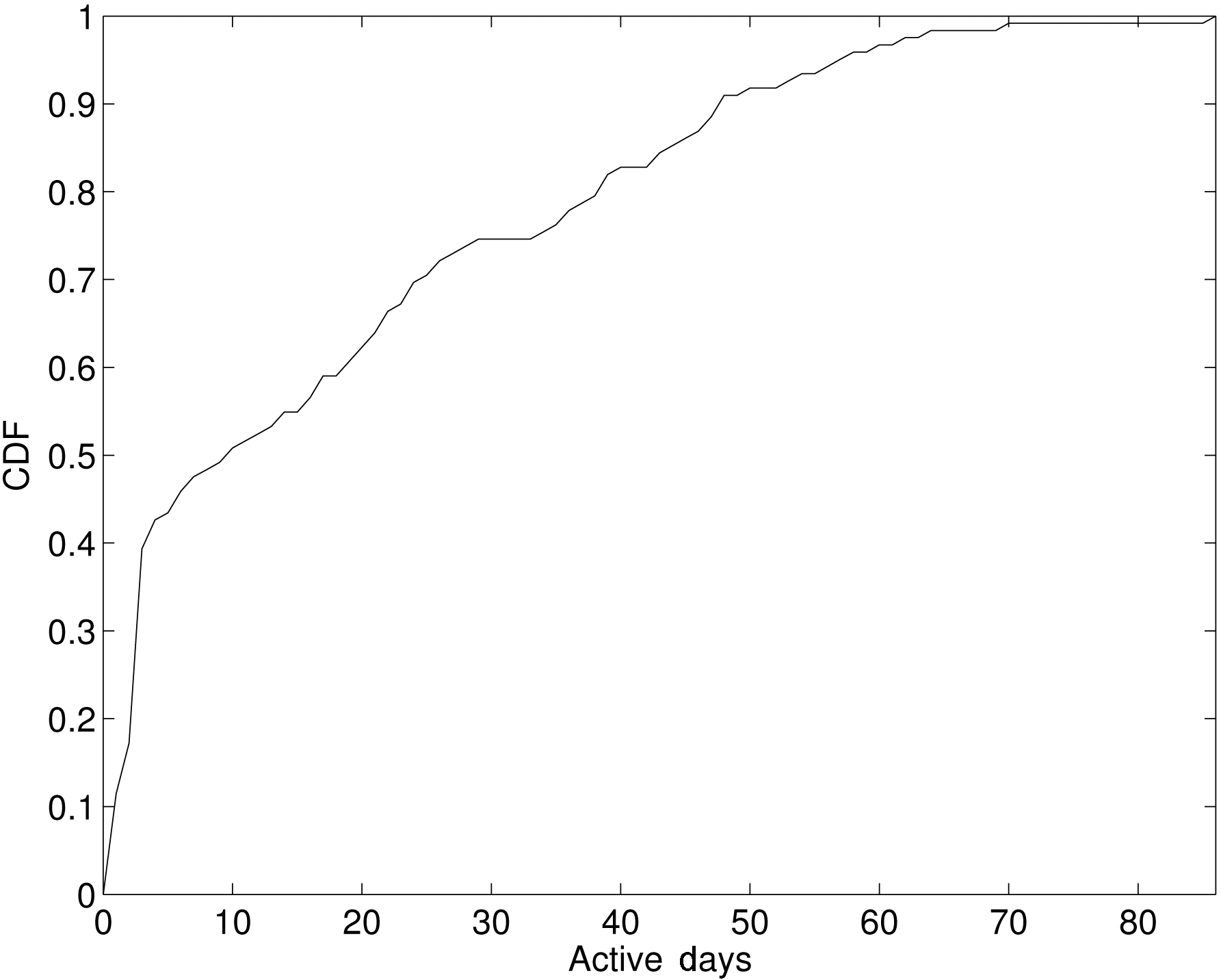
In our trace, we have 124 VoIP users. While some users are regular users who were active most days, the rest did not use their device regularly. In our analysis, we focused on the regular users, defined as users who connected to any access point more than seven days during the three-month period. We found 64 users (52%) to be regular. Figure 2 shows the CDF of the number of active days across 124 users.
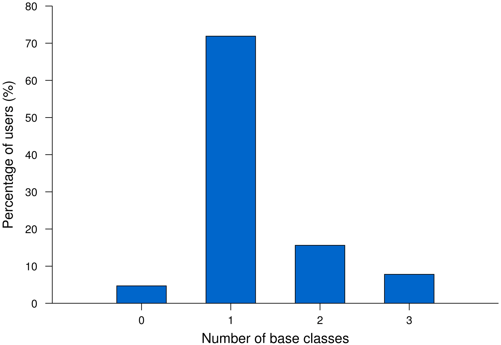
We applied our classification mechanism to 64 regular users. For each user, our system classified only the active user days. Recall that our system created a class whenever a new user-day trace could not be classified into one of the existing classes. We called any class that contained five or more user-days a baseclass. Figure 3 shows the histogram of users with a different number of base classes. 71.9% of users had only one base class during the three month period, while 23.4% had more than one base class.
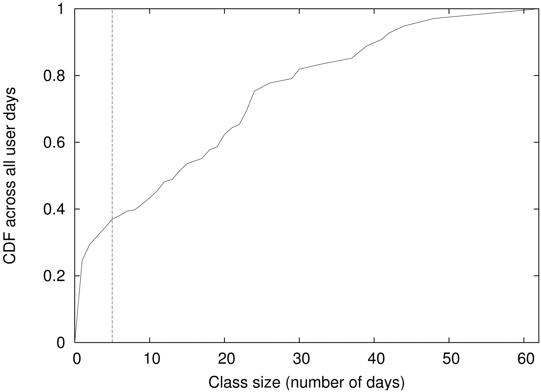
We first needed to understand the percentage of user days that could be considered as regular versus unusual. Figure 4 shows the CDF across all user days. The x-axis
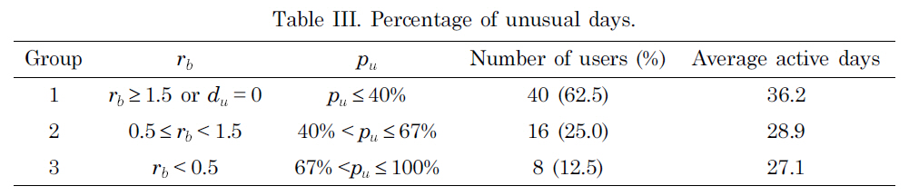
[Table 3.] Percentage of unusual days.

Percentage of unusual days.
shows the class size in terms of days and the y-axis shows the cumulative percentage of days that belong to a class with a specific size. First, using our threshold of 5 days to be considered as a base class, we found that 34% (731 days) of user days were considered to be unusual. If we reduced the threshold, the percentage of unusual days would reduce. We chose the default threshold to be a little smaller than the cut off for identifying the active users. Since we focused on the users who were active more than 7 days, we chose our threshold to be 5 days. Second, the majority of unusual days were a one-time event. In other words, the mobility pattern did not repeat. Among all the unusual days, 72% belonged to a class of size 1 (day).
We then considered how many of the active users had a regular mobility pattern. To quantify this, we defined rb as the ratio of the number of days that belonged to base classes (
Table III shows
group. Group 1, whose days mostly belonged to a base class, had the largest number of active days (36.2 days). The other two groups had a smaller number of active days than that of Group 1, but they were still large enough to have a base class (5 days).
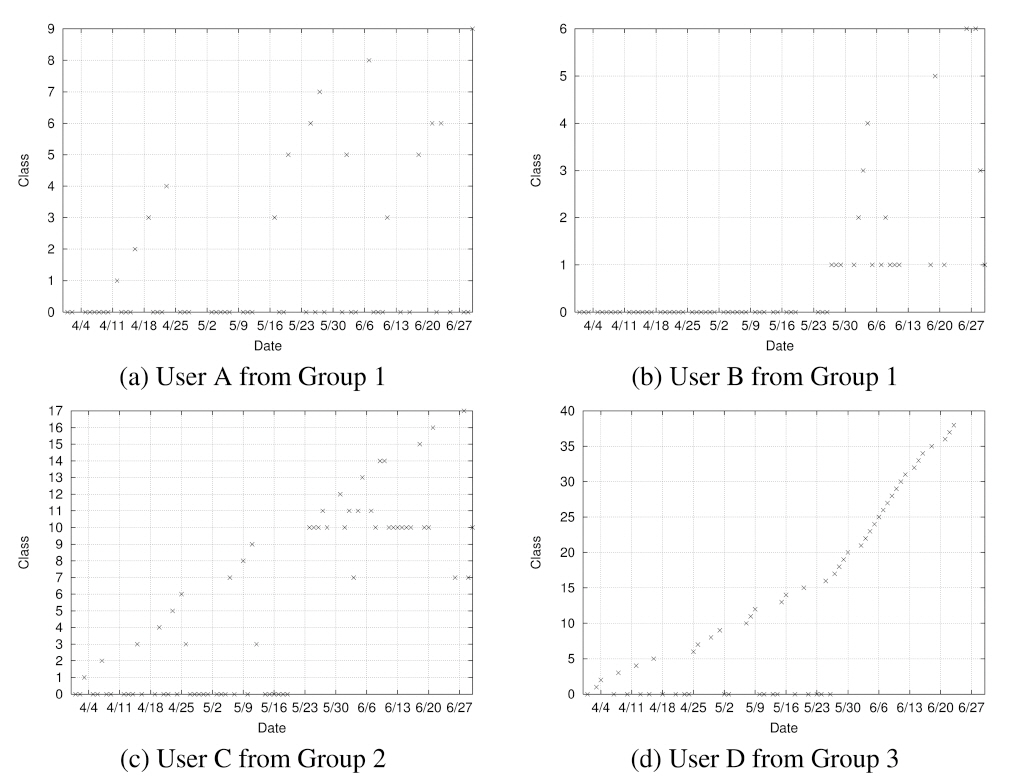
Figure 5 shows the class assignment across three months for several sample users extracted from each of the three groups of Table III. The x-axis shows time and the y-axis shows the class into which the mobility pattern of the particular day falls. Note that the dates labeled on the x-axis (and drawn with grid lines) denote Sundays. User A had only one base class (Class 0) and the majority of his or her days belonged to this class. User B had two base classes (Class 0 and 1) and again a majority belonged to these base classes. In User C’s case, roughly half belonged to base classes. A majority of User D’s days did not belong to a base class.
Through this study, we also discovered several interesting mobility characteristics. First, we did not observe any repeating pattern based on the day of the week. The only weekly pattern that we observed was that most users were active during only the week days and not active during weekends (User A and B in Figure 5). Second, a change in mobility patterns coincided with an academic calendar. For a set of users, their mobility pattern was regular during academic terms but became irregular during summer vacation. For the first two months, these users had a base class and
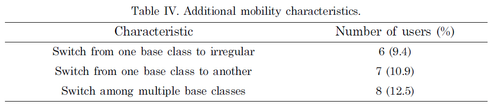
[Table 4.] Additional mobility characteristics.

Additional mobility characteristics.
most of their days belonged to this base class. Then, toward the end of May, which is when the term ended for that academic year at Dartmouth, these users’ days did not belong to any base class (User D). For another set of users, their mobility pattern shifted from one base class to another towards the end of May (User C). Third, while most users had one base class, some users had multiple base classes, often switching back and forth among them.
The mobility characteristics are important to understand for pervasive application developers during their design and testing. For example, to test new software in a simulation environment, they need to know how many users follow certain characteristics. Table IV shows the number of users that followed the mobility characteristics described above. Note that the first observation applied to most users and thus we did not include it in this table.
In summary, we identified unusual days using Pearson’s test. If r did not exceed the critical value, then the corresponding day was considered to be different from usual days (which belonged to one of base classes). However, for those users who did not show any regular mobility patterns, we could not identify any unusual days since there were no regular or usual days.
In the previous section, we identified many interesting mobility characteristics of individual users using our system. In this section, we look into some unusual days that we identified in the previous section to deepen our understanding of the findings.
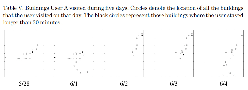
We first considered five active days of User A in detail: 5/28, 6/1, 6/2, 6/3, and 6/4. Among these five days, only 6/2 was identified as a different class (See the graph in Figure 5). Table V depicts the locations of buildings (on an invisible campus map) that User A visited on each day. Each circle shows a building and the filled circles show

Buildings User A visited during five days. Circles denote the location of all the buildings that the user visited on that day. The black circles represent those buildings where the user stayed longer than 30 minutes.
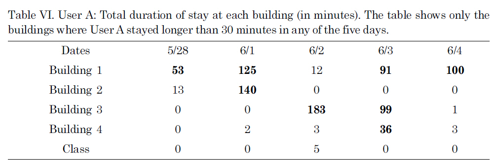
User A: Total duration of stay at each building (in minutes). The table shows only the buildings where User A stayed longer than 30 minutes in any of the five days.

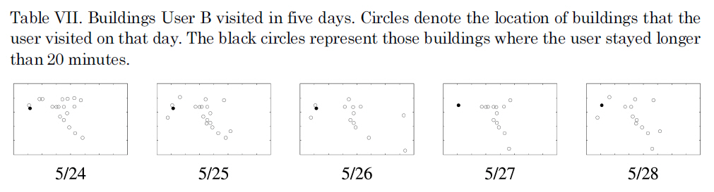
Buildings User B visited in five days. Circles denote the location of buildings that the user visited on that day. The black circles represent those buildings where the user stayed longer than 20 minutes.
those buildings where the user stayed longer than 30 minutes. Note that our system used both the location and time information, while this figure shows only the location without the exact duration of stays. For a better understanding of why 6/2 was classified into a different class, we also showed the duration of stay at buildings (where the user stayed for more than 30 minutes total) in Table VI. From Table VI, we can clearly see that User A spent much more time at Building 1 on those four days (in Class 0) while she did not visit Building 1 and stayed mostly in Building 3 on 6/2 (in Class 5).
Another case that we considered was class transition. User B in Figure 5 shows a class transition during the week of 5/23. Days up to 5/26 belong to Class 0 and the days after that belong to Class 1. Table VII shows the buildings that User B visited in five days: 5/24, 5/25, 5/26, 5/27, and 5/28. The circles show the location of the buildings and filled circles show the buildings where users spent more than 20 minutes. Table VIII shows the duration of stay at the two buildings. It is clear how the days are classified into two different classes. User B stayed at Building 5 in the beginning of the trace and then stayed mostly in Building 6.
In summary, as illustrated with sample users, we could easily do the following using our system:
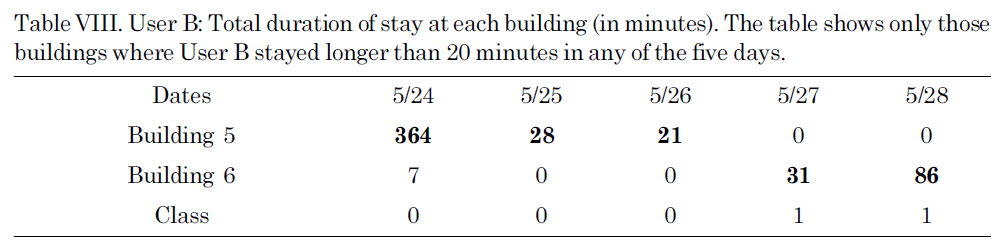
User B: Total duration of stay at each building (in minutes). The table shows only those buildings where User B stayed longer than 20 minutes in any of the five days.
Identify days when mobility patterns change.
Identify days where the pattern looks like that of many other days, i.e., a typical day.
Identify days where the pattern does not look like (many) other days, i.e., an unusual day.
Discover the general characteristics of human mobility.
5. SAMPLE APPLICATION SCENARIO
In this section, we introduce a sample pervasive application and how our mechanism interacts with this application.
Digital memories or diaries often use a body-mounted camera to capture photos or movie streams. Because this data can quickly accumulate, it is important to distill or compress the data. One simple way to distill the data would be to filter out data frames or photos at fixed intervals. However, this static method of distillation would lose many details that the user may later find interesting. Perhaps distillation should be done differently if a certain day was special or interesting. For many people whose jobs did not vary much from day to day, the system probably would not record many new things every day. A typical day for such people would be images of home, the route to work, and the office. However, when a person takes a vacation and travels, the camera is likely to capture many new images. Thus, the distillation system should capture these special days and apply different filters to the data according to type of days that the data was gathered.
We now consider this application in more detail and how it interacts with our system. The head-mounted camera captures images during the day. Locations of the user are also recorded. At the end of the day, the user backs up the data to a storage server. For a fixed time period, the server keeps the original data. When the data is about to expire, the server needs to decide how to distill the data. To make the decision, the server sends location information to our system, and our system determines the significance of that day. The significance level may be either determined using a system default (e.g., highest level for the first day of a class) or predefined by the user. Our system returns the significance level to the server and the distillation server compresses data according to the significance level.
Although our current system detects unusual days solely based on mobility patterns, we recognize that we ultimately need to combine other contextual information to detect unusual days. For example, an office worker may spend the usual amount of time in the usual places, but something about their work that day (such as the people they met, conversations they had, or tasks they performed) may have been unusual. We can adapt other sensor-based systems to collect different categories of information. For example, activity recognition systems [Consolvo et al. 2008, Choudhury et al.2008] may provide a series of activity data, and this data can be put into our detection system to identify unusual activities. Using both activities and mobility patterns, we can identify unusual days that may be more meaningful to users.
Numerous pervasive applications such as digital memories collect a large amount of data now that sensing devices and storage are both cheap and readily available. One key challenge is to identify and retrieve interesting data. In this paper, we presented a system that automatically identified unusual days using location information. We evaluated our detection system using real wireless-network traces collected on the Dartmouth campus. Our system identified regular mobility patterns, detected changes in the patterns, identified unusual days, and also extracted general characteristics of human mobility. Although we evaluated our system using wireless-network traces, we expect that other types of location information would also be easy to collect using devices such as GPS.
In the future, we would like to develop a distillation application for digital memories as described in Section 5, and use our system for indexing and adaptive distillation. We would then collect image data along with location information and use our system to effectively manage the vast amount of image data.