Privacy preserving microdata publication has received wide attention [1-5]. Each record corresponding to one individual has a number of attributes, which can be divided into the following three categories: 1)
Before microdata are released, identity attributes are often directly removed to preserve privacy of individuals whose data are in the released table. However, the
The randomization approach has also been adopted to publish microdata [8-12]. Instead of generalizing
Our contributions are summarized as follows. We present a systematic study of the randomization method in preventing attribute disclosure under linking attacks. We propose the use of a specific randomization model and present an efficient solution to derive distortion parameters to satisfy requirements for privacy preservation, while maximizing data utilities. We propose a general framework and present a uniform definition for attribute disclosure which is compatible for both randomization and generalization models. We compare our randomization approach with
The remainder of this paper is organized as follows. In Section II, we discuss closely related work on group based anonymization approaches and randomization approaches in privacy preservation data publishing. In Section III, we present background on randomization based distortions, including analysis and attacks on the randomized data. In Section IV, we first quantify attribute disclosure under linking attacks and then show our theoretical results on maximizing utility with privacy constraints. In Section V, we conduct empirical evaluations and compare the randomization based distortion with two representative group based anonymization approaches (
>
A. Group Based Anonymization
Kifer and Gehrke [15] investigated the problem of injecting additional information into k-anonymous and
In this paper, we focus on the randomization model in resisting attribute disclosure of data publishing. The proposed randomization model is compared to traditional
The first randomization model, called Randomized Response(RR), was proposed by Warner [28] in 1965. The model deals with one dichotomous attribute, i.e., every person in the population belongs either to a sensitive group
Aggarwal and Yu [30] provided a survey of randomization models for privacy preservation data mining, including various reconstruction methods for randomization, adversarial attacks,optimality and utility of randomization. Rizvi and Haritsa [9]developed the MASK technique to preserve privacy for frequent item set mining. Agrawal and Haritsa [31] presented a general framework of random perturbation in privacy preservation data mining. Du and Zhan [8] studied the use of a randomized response technique to build decision tree classifiers. Guo et al. [10] investigated data utility in terms of the accuracy of reconstructed measures in privacy preservation market basket data analysis. Aggarwal [32] proposed adding noise from a specified distribution to produce a probabilistic model of k-anonymity.Zhu and Liu [33] investigated the construction of optimal randomization schemes for privacy preservation density estimation and proposed a general framework for randomization using mixture models. Rebollo-Monedero et al. [34]defined the privacy measure similar to t-closeness [7] and formalized the privacy-utility tradeoff from the information theory perspective. The resulting solution turns out to be the postrandomization(PRAM) method [35] in the discrete case and a form of random noise addition in the general case. They also proved that the optimal perturbation is in general randomized,rather than deterministic in the continuous case.
Huang and Du [36] studied the search of optimal distortion parameters to balance privacy and utility. They developed an evolutionary multi-objective optimization method to find optimal distortion matrices when applying the RR technique on a single attribute. The complexity of the algorithm is
In our paper, we focus on a specific randomization model(i.e., perturbation retains the original value of an attribute
Dataset
Attribute
Let πi1, … , i m, isdenote the true proportion corresponding to the categorical combination (A1 = i1, · · · , Am = im, S = is). Let πi1be the column vector with
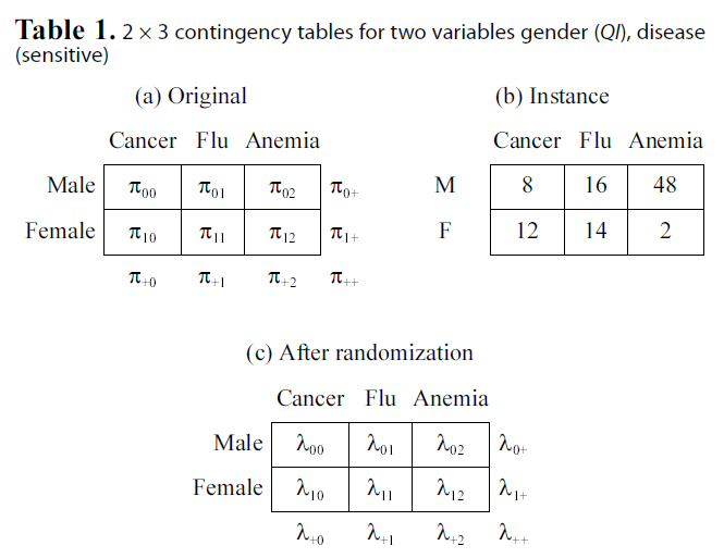
[Table 1.] 2 × 3 contingency tables for two variables gender (QI) disease(sensitive)

2 × 3 contingency tables for two variables gender (QI) disease(sensitive)
categorical attributes. Results of most data mining tasks (e.g.,clustering, decision tree learning, and association rule mining),as well as aggregate queries, are solely determined by the contingency table. That is, analysis on contingency tables is equivalent to analysis on the original categorical data. Table 1b shows one contingency table instance derived from the data set with 100 tuples. We will use this contingency table as an example to illustrate properties of link disclosure.
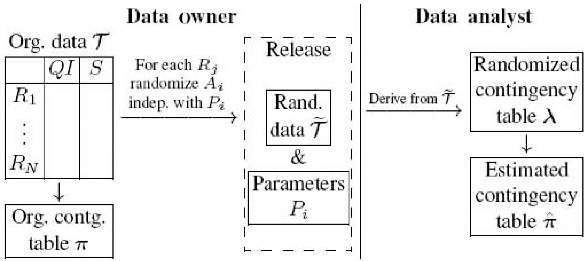
We use the left part of Fig. 1 to illustrate the process of privacy preserving data publishing. For each record
Let λ denote the contingency table of the randomized data
Distortion matrices determine the privacy and utility of the randomized data. How to find optimal distortion parameters with privacy or utility constraints has remained a challenging problem [39]. In this paper, we limit the choice of randomization parameters for each
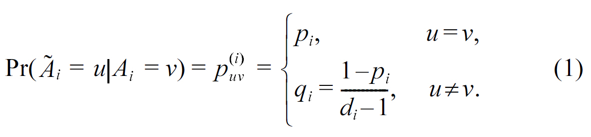
That is, for each attribute
>
B. Analysis on the Randomized Data
One advantage of randomization procedure is that the pure random process allows data analysts to estimate the original data distribution based on the released data and the randomization parameters. The right part of Fig. 1 shows how data analysts estimate the original data distribution. With the randomized data
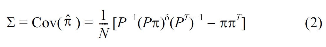
where (Pπ)δ stands for the diagonal matrix, whose diagonal values are Pπ.
Thus, data analysts derive the estimation for the distribution of original data (in terms of contingency table) without disclosing the individual information of each record. We choose the accuracy of reconstructed distribution as the target utility function in Section IV-B, because most data mining applications are based on the probability distribution of the data.
>
C. Attacks on Randomized Data
Let

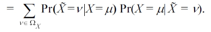
where Pr(X =
The following lemma gives the accuracy of the attacker’s estimation.
LEMMA 1.
PROOF. For a particular observed value X =
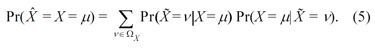
The probability of attackers’ correct estimation is also defined as the reconstruction probability, Pr(
IV. ATTRIBUTE DISCLOSURE UNDER LINKING ATTACKS
We measure privacy in terms of the attribute disclosure risk,whose formal definition is given, as follows:
DEFINITION 1.
We need to quantify the background knowledge of attackers to derive the disclosure probability Pr(
>
A. Quantifying Attribute Disclosure
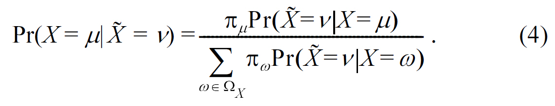
When there is no randomization applied, for those records with their quasi-identifiers equal to

because there are πQIr records within the group of
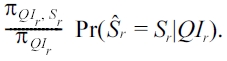
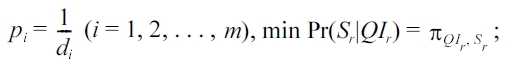
1) Randomize S only (RR-S): When data owners only apply randomization to the sensitive attribute, for each record within the group of QIr, the attacker takes a guess on its sensitive value using the observed sensitive value and the posterior probability in (4). According to (5), the probability of a correct estimation is Pr( = ?r'QIr), then the risk of sensitive attribute disclosure is
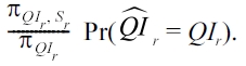
2) Randomize QI only (RR-QI): Similarly as RR-S, when data owners only apply randomization to the quasi-identifiers,the probability of correctly reconstructing QIr is given by Pr(Xr= QIr), and hence the risk of sensitive attribute disclosure is
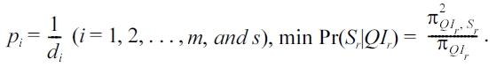
3) Randomize QI and S (RR-Both): When data owners apply randomization to both QI and S, the attacker first needs to ensure the values of identifier attributes are correctly reconstructed.The probability is given by Pr(QIr = QIr). Second, the attacker needs to ensure the value of the sensitive attribute,given the correctly reconstructed identifier attribute values are correctly reconstructed. We summarize the risk of sensitive attribute disclosure in RR-Both , as well as RR-S and RR-QI, in the following result and give the general calculation of the attribute disclosure risk in the randomization settings.
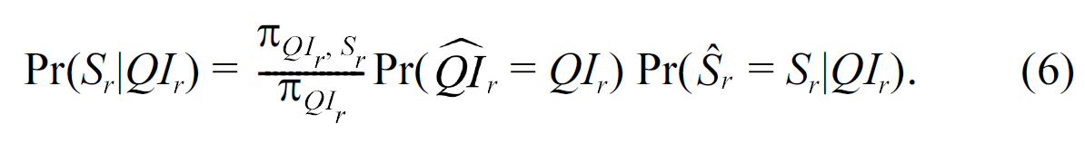
We give the formal expressions of the two reconstruction probabilities needed in calculating Pr(
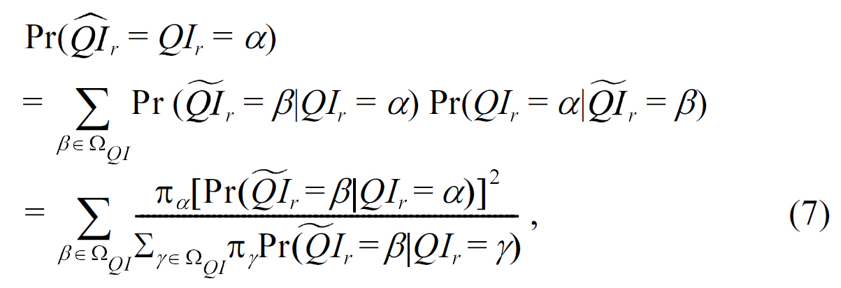
where Pr(QI~r =
is the probability that α ={
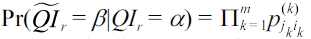
The reconstruction probability of the sensitive attribute
We are interested in when the attribute disclosure reaches the minimum. We show our results in the following property and include our proof in the Appendix.
for RR-
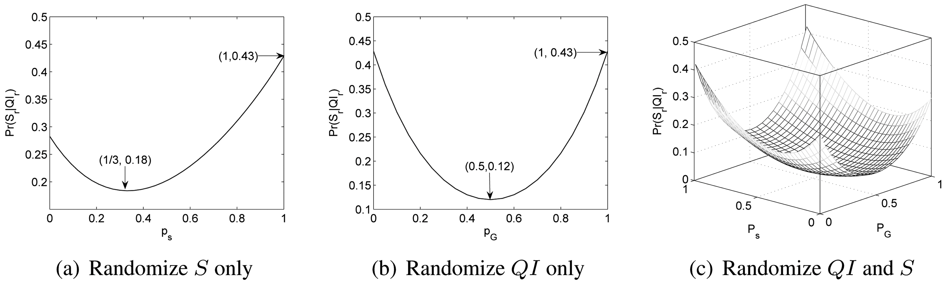
Example. We use the instance shown in Table 1b to illustrate this property. For an individual r with (

when no randomization is introduced. Fig. 2a shows the scenario when
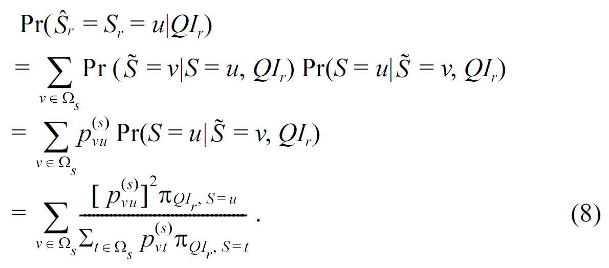
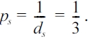
we only randomize S. We can see that min
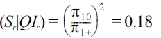
when Ps = 1/ds = 1/3s
Fig. 2b shows the scenario when we only randomize
Fig. 2c shows the case where randomization is applied to both
Computational Cost.The main computation cost in (6)comes from calculating Pr(
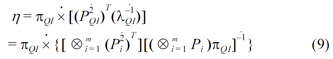
where × denotes the component-wise multiplication, P
In (9), we need to repeatedly calculate (P1 ? · · · ? Pm)
LEMMA 2.
(
Applying Lemma 2 recursively, we can reduce the time complexity to
contingency table.
>
B. Maximizing Utility with Privacy Constraints
The ultimate goal of publishing data is to maximize utility,while the minimizing risk of attribute disclosure simultaneously.The utility of any data set, whether randomized or not,is innately dependent on the tasks that one may perform on it.Without a workload context, it is difficult to say whether a data set is useful or not. This motivates us to focus on the data distribution when evaluating the utility of a database, since many data mining applications are based on the probability distribution of the data.
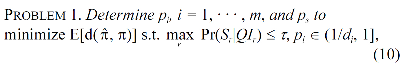
We can set the privacy threshold formalize as the same privacy requirement of l-diversity (i.e., τ = 1/
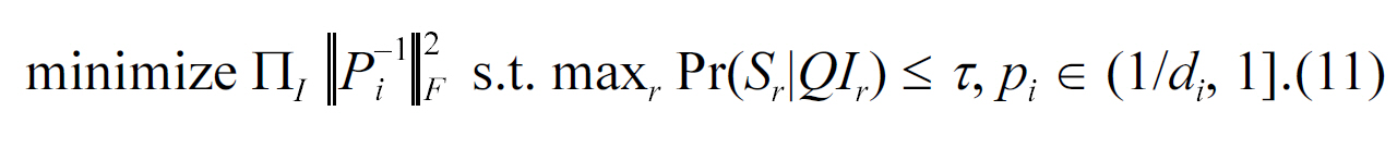
Problem 1 is a nonlinear optimization problem. In general,we can solve it using optimization packages (e.g., trust region algorithm [40]). In Section IV-A, we discussed how to efficiently calculate the attribute disclosure of target individuals(shown as constraints in PROBLEM 1). Next, we show how we can efficiently calculate
RESULT 2.
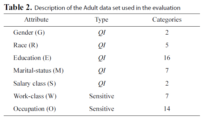
[Table 2.] Description of the Adult data set used in the evaluation

Description of the Adult data set used in the evaluation
squared Euclidean distance, with Lemma (3) shown in the Appendix, to minimize d(X, π) is equivalent to minimize trace(Σ) where Σ is the covariance matrix of the estimator of cell values in the contingency table (shown in Equation 2). Calculating trace(Σ) still involves high computational cost. However,when
where 1 is the column vector whose cells are all equal to 1.
We ran our experiments on the Adult Database from the UCI data mining repository [41] in our evaluations. The same database has been used in previous work on
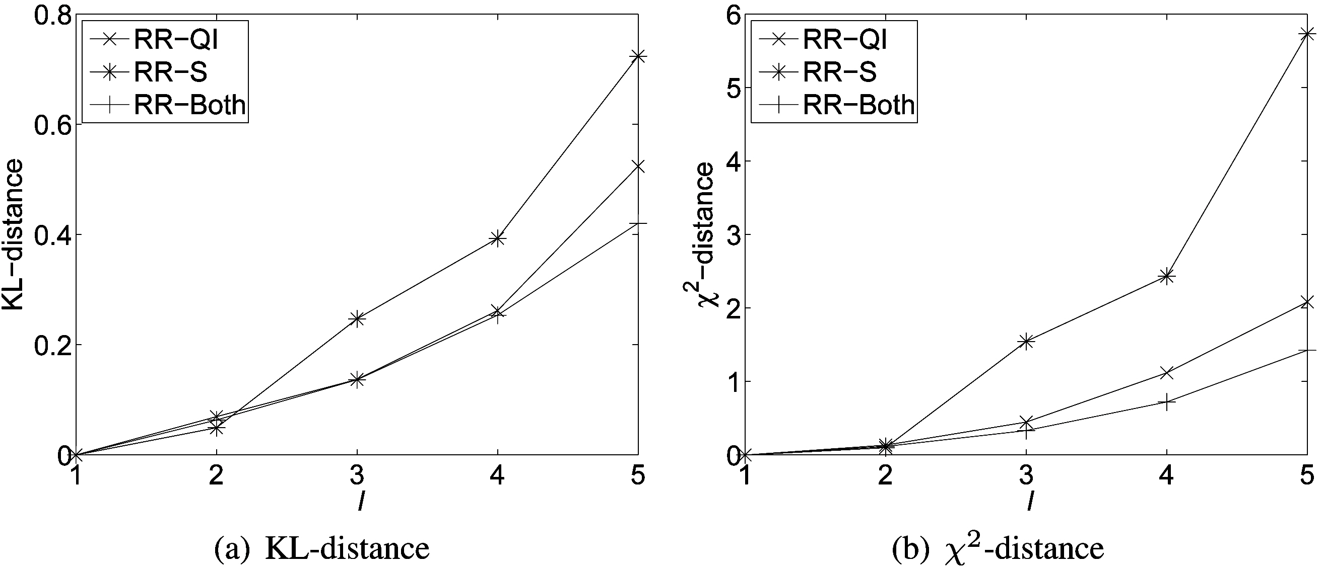
It is expected that a good publication method should preserve both privacy and data utility. We set different l values as privacy disclosure thresholds. We adopt the following standard distance measures to compare the difference of distributions between the original and reconstructed data to quantify the utility. Given two distributions
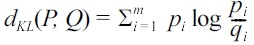
and
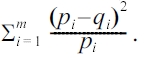
In our evaluation, we first investigate utility vs. privacy of the randomization method in protecting attribute disclosure on two aspects: 1) compare data utility among different scenarios,and 2) the impact of cardinality upon data utility. Then, we compare randomization with
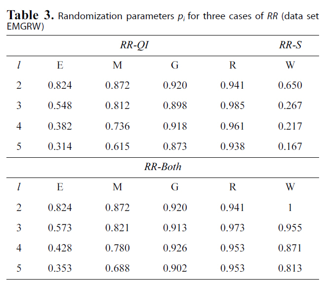
[Table 3.] Randomization parameters pi for three cases of RR (data setEMGRW)

Randomization parameters pi for three cases of RR (data setEMGRW)
We treated
Fig. 3 shows results on various distance measures. Naturally,there is a tradeoff between minimizing utility loss and maximizing privacy protection. Fig. 3 indicates that the smaller the distance values, the smaller the difference between the distorted and the original databases, and the better the utility of the distorted database. We can observe that the utility loss (in terms of distance differences) increases approximately linearly with the increasing privacy protection across all three randomization scenarios.
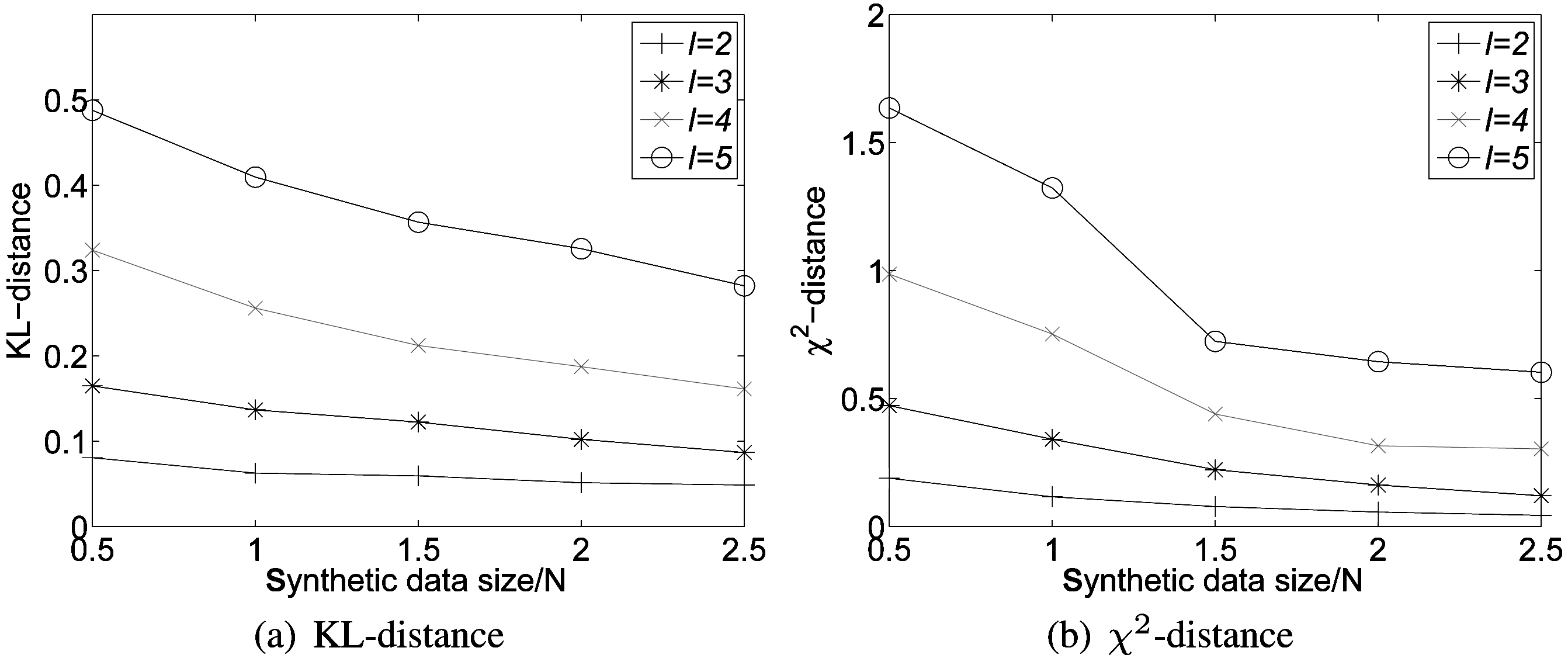
As discussed in Section III, one advantage of the randomization scheme is that the more data we have, the more accurate reconstruction we can achieve. We generate four more data sets with varied sizes by sampling
>
B. Comparison to Other Models
We chose
Generalization approaches usually measure the utility syntactically by the number of generalization steps applied to quasi-identifiers [42], average size of quasi-identifier equivalence classes [2], sum of squares of class sizes, or preservation of marginals [3]. We further examine the utility preservation from the perspective of answering aggregate queries, in addition to the previous distribution distance measures, since the randomization scheme is not based on generalization or suppression.We adopt query answering accuracy; the same metric is used in Zhang et al. [4]. We also consider the variation of correlations between the sensitive attribute and quasi-identifiers. We used an implementation of the Incognito algorithm [3] to generate the entropy
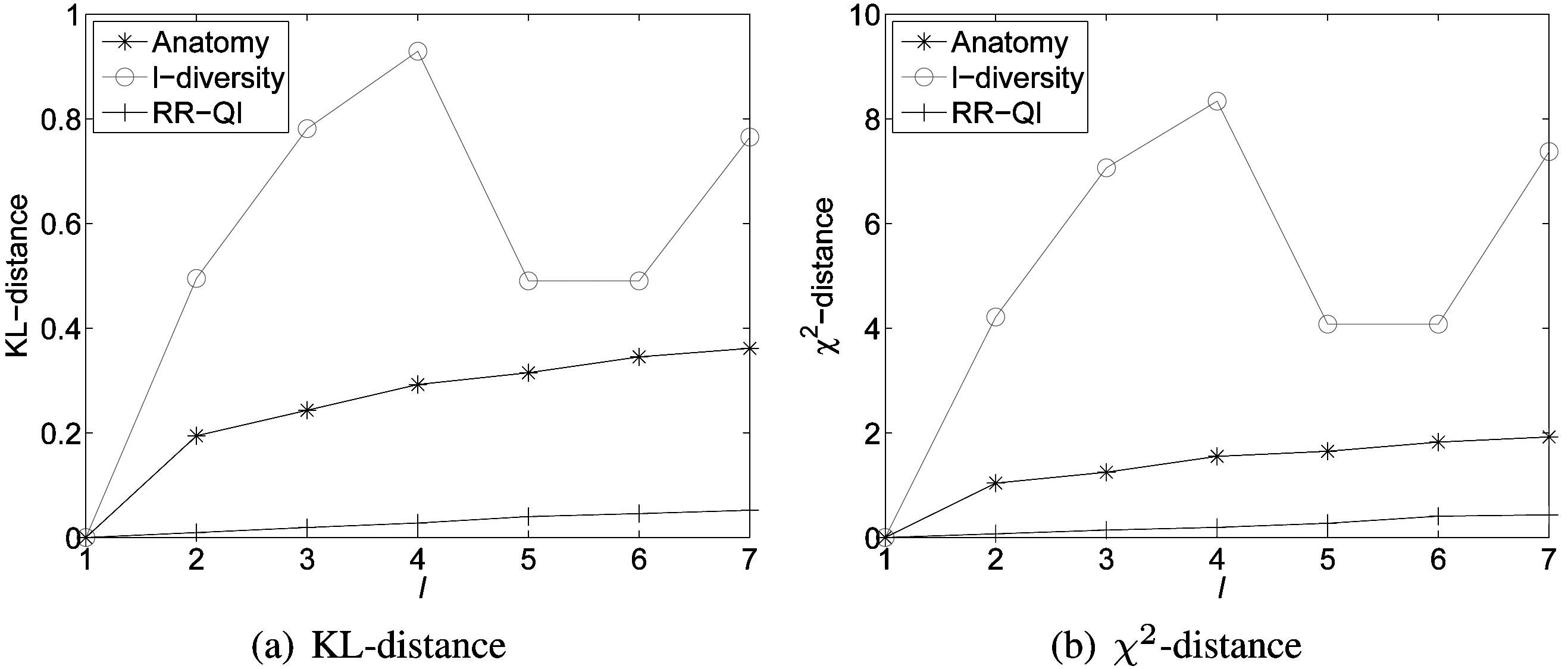
1) Distribution Distance: We compare data utility of reconstructed probability distributions for different models according to the distance measures. Fig. 5 shows distances between X and π for anatomy, l-diversity and RR-QI on the data set ESGRO.We can observe that randomization outperforms both anatomy and l-diversity methods, because we can partially recover the original data distribution in the randomization scheme, whereas data distribution within each generalized equivalence class is lost in l-diversity generalization and the relations between the quasi-identifier table (QIT) and the sensitive table (ST) are also lost in anatomy.
Another observation is that data utility (in terms of distance between original and reconstructed distributions) monotonically decreases with the increment of the privacy thresholds (l) for randomization and anatomy. This is naturally expected, because more randomness needs to be introduced with the increment of the privacy requirements for randomization and larger l in anatomy means that more tuples are included in each group, which decreases the accuracy of the estimate for the distribution of the original data. However, there is no similar monotonic trend in l-diversity,because the generalization algorithm chooses different attributes for generalization with various l values; this makes the accuracy of the estimated distribution vary to different extents.
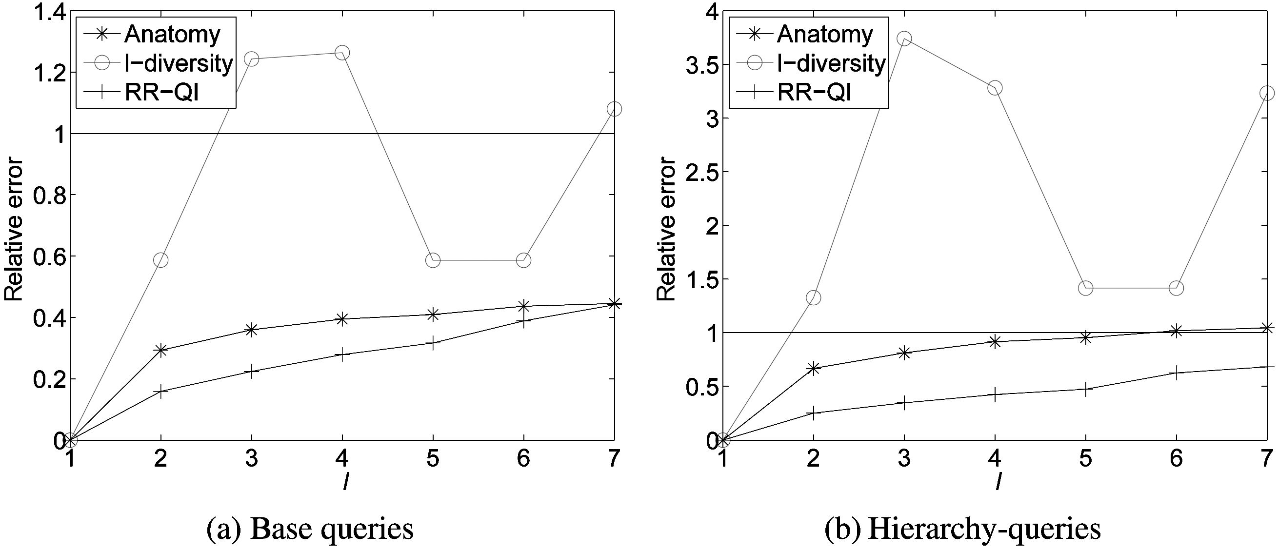
2) Query Answering Accuracy:The accuracy of answering aggregate queries is one of the important aspects to evaluate the utility of distorted data. We compare randomization against two other anonymization approaches [3, 5] using the average relative error in the returned count values. For each count value(corresponding to the number of records in a group), its relative error is defined as |act - est|/act, where act is the actual count value from the original data, and est is the estimate from the reconstructed data for RR approaches or the anonymized data for anonymization approaches. We consider two types of queries in our evaluation.
- Base group-by query with the form:SELECT A1,. . . , Am, S, COUNT(*) FROM data
WHERE A1 = i1 . . . Am = im AND S = is GROUP BY (A1, · · · ,
Am, S)
Where ik ∈ Ωk and is ∈ Ωs.
- Cube query with the form:
SELECT A1,· · · , Am, S, COUNT(*) FROM data
GROUP BY CUBE (A1, · · · , Am, S)
The base group-by query returns the number of records in each group of (
After running the base group-by query on the original data and the reconstructed data or the anonymized data, we get the count values of act and est, respectively. Fig. 6a shows the calculated average relative errors of three methods (anatomy,
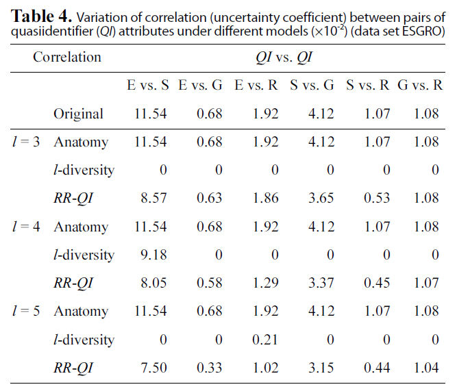
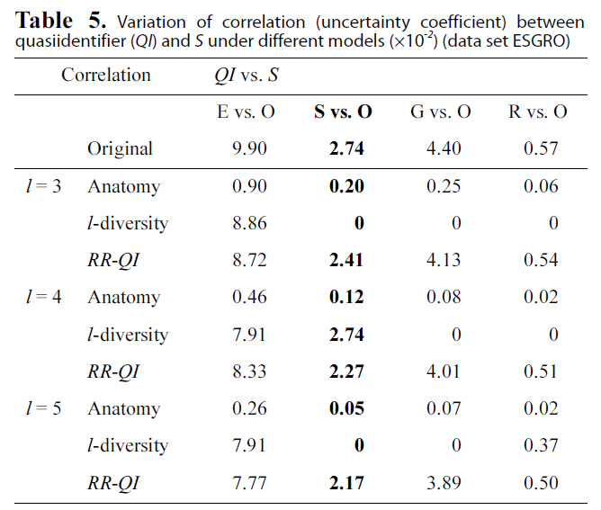
3) Correlation Between Attributes: A good publishing method should also preserve data correlation (especially between QI and sensitive attributes). We use Uncertainty Coefficient(U) to evaluate the correlation between two multi-category variables:
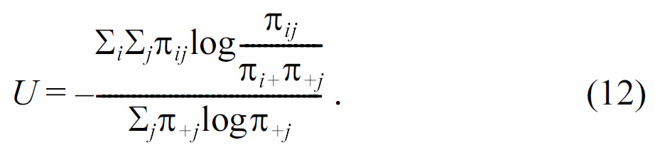
The uncertainty coefficient takes values between -1 and 1;larger values represent a strong association between variables.When the response variable has several possible categorizations,these measures tend to take smaller values, as the number of categories increases.
Table. 4 and 5 show correlation (uncertainty coefficient) val-

Variation of correlation (uncertainty coefficient) between pairs ofquasiidentifier (QI) attributes under different models (×10-2) (data set ESGRO)

Variation of correlation (uncertainty coefficient) betweenquasiidentifier (QI) and S under different models (×10-2) (data set ESGRO)
ues between each pair of attributes vary under three models(anatomy,
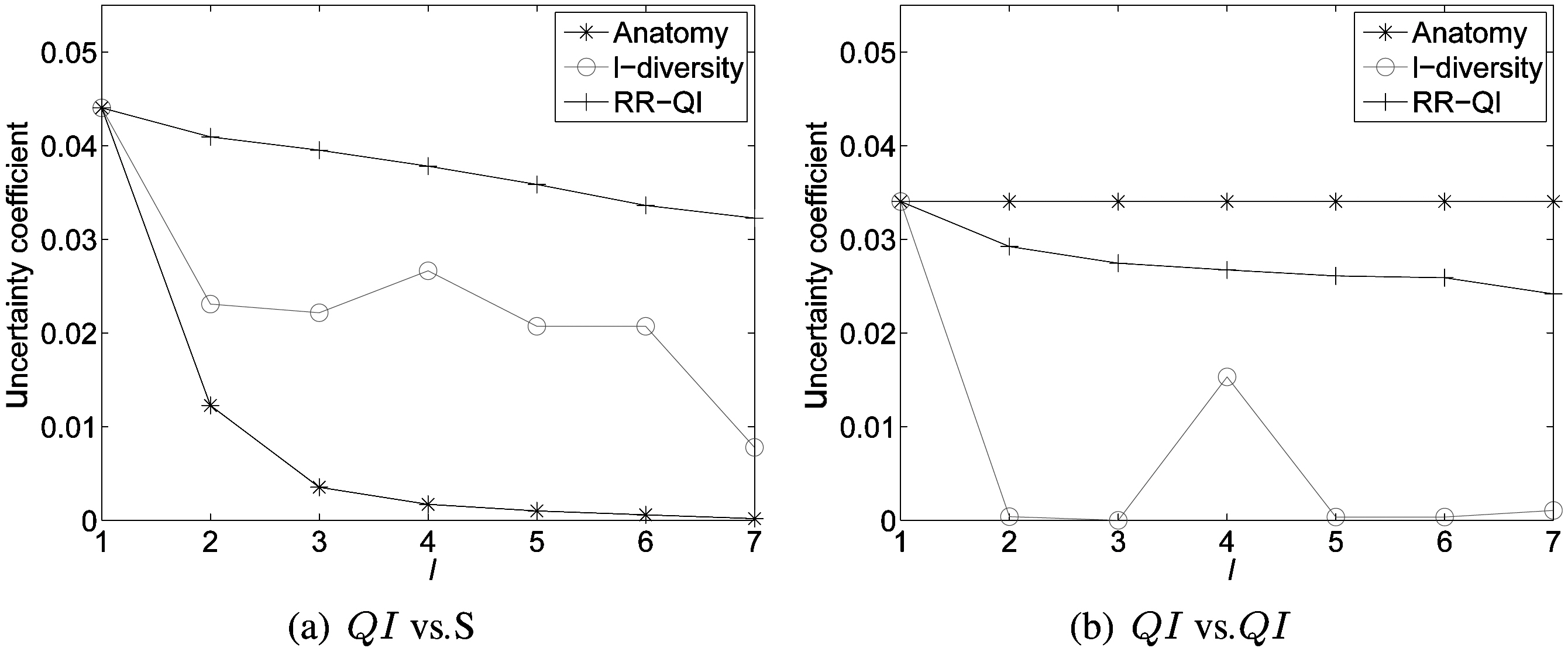
Fig. 7 shows the average value of uncertainty coefficients among attributes for anatomy, l-diversity and RR-Both on the data set ESGRO. As shown in Fig. 7a, randomization achieves the best correlation preservation between the sensitive attribute and quasiidentifiers across all privacy thresholds. Fig. 7b also clearly shows that randomization better preserves correlation among quasi-identifiers than l-diversity does. Please note that anatomy can best achieve the correlation among quasi-identifiers,since it does not change values of quasi-identifiers.
In summary, the evaluation shows that randomization can better preserve utility (in terms of distribution reconstruction,accuracy of aggregate query answering, and correlation among attributes) under the same privacy requirements. Utility loss is significantly smaller than that of generalization or anatomy approaches. Furthermore, the effectiveness of randomization can be further improved when more data are available. The evaluation also showed that the randomization approach can further improve the accuracy of the reconstructed distribution(and hence utility preservation) when more data are available,while generalization and anatomy approaches do not have this property.
In this paper, we investigated attribute disclosure in the case of linking attacks. We compared randomization to other anonymization schemes (l-diversity and anatomy) in terms of utility preservation, with the same privacy protection requirements.Our experimental evaluations showed randomization significantly outperforms generalization, i.e., achieving better utility preservation, while yielding the same privacy protection.
There are several other avenues for future work. We aim to extend our research to handle multiple sensitive attributes. In this paper, we limit our scope, as attackers have no knowledge about the sensitive attribute of specific individuals in the population and/or the table. In practice, this may not be true, since the attacker may have instance-level background knowledge(e.g., the attacker might know that the target individual does not have cancer; or the attacker might know complete information about some people in the table other than the target individual.)or partial demographic background knowledge about the distribution of sensitive and insensitive attributes in the population.Different forms of background knowledge have been studied in privacy preservation data publishing recently. For example, the formal language [22, 24] and maximum estimation constraints[43] are proposed to express background knowledge of attackers.We will investigate privacy disclosure under those background knowledge attacks. We should note that randomization may not outperform generalization in all cases, especially when some specific background knowledge is utilized in the adversary model, because generalization is truthful and the ambiguity is between true tuples (e.g., individual a and b are indistinguishable),whereas randomization can be regarded as adding noise,and noise can be removed when some background knowledge is known.
We will continue our study of further reducing computation overhead of the randomization approach. The execution time of randomization is usually slower than l-diversity and anatomy.For example, the execution time of our RR-Both approach on the Adult data sets was 10 times slower than for generalization approaches due to the heavy cost of determining the optimal distortion parameters with attribute disclosure constraints, especially when the attribute domains are large. One advantage of randomization is that the reconstruction accuracy increases when more data are available. Guo et al. [10] preliminarily conducted theoretical analysis on how the randomization process affects the accuracy of various measures (e.g., support, confidence,and lift) in market basket data analysis. In our future work, we will study the accuracy of reconstruction in terms of bias and variance of estimates in randomizing general microdata.
Finally, we are interested in comparing our randomization approaches to most recently developed generalization approaches(e.g., the accuracy-constrained l-diversification method in [14]).We are also interested in combining the derived optimal randomization schemes with the small domain randomization [38]to further improve utility preservation. It is our belief that extensive studies on comparing different privacy preservation data publishing approaches are crucial.
>
Appendix 1. Proof of Property 1
We start with applying RR to the sensitive attribute, Pr( r =QI^r) = 1. Without loss of generality, we assume that Sr = 1. Combine other categories 0, 2, . . . , ds - 1 into a new categories, and still use 0 to denote the new category. To make the notation simple,we simply write

as π0 in this proof, then π1 =1 ? π0. Such adjustment does not change the reconstruction probability Pr( S?r = Sr = 1'QIr). After the adjustment, the randomization probabilities are given by

By definition, the posterior probabilities are given by
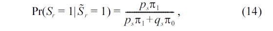
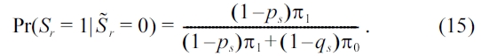
Combining (13), (14), and (15), we have
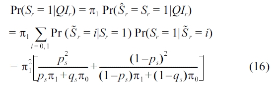
Taking the derivative with respect to ps, we have (16) is minimized when ps = 1/ds , and the minimal value is
Following similar strategies, we can prove the general case when we randomize both QI and S.
>
Appendix 2. Proof of Result 2
LEMMA 3. If d( π^ , π) = '' π^ π''22 , we have E[d( π^, π)] = trace(Σ), where Σ is the covariance matrix of π^ shown in (2).
PROOF. We know that π^ asymptotically follows the normal distribution N(π, Σ). Let Σ = XΛXT be the eigen-decomposition of Σ, where Λ = diag(λ1, . . . , λn) and XTX = I. Let η = XT (π^ π), then η is normally distributed with E(η) = 0 and
Cov(η) = XT Cov( π^ π)X = XTΣX = Λ.
Notice that Λ is a diagonal matrix, and hence Cov(ηiηj) = 0 if i ≠ j, and Var(ηi) = λi, i.e., ηi independently follows the normal distribution N(0, λi). Therefore, we have:
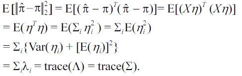
The last equality is due to the fact that
trace(Σ) = trace(XΛXT) = trace(ΛXTX) = trace(Λ).
We proved the lemma.
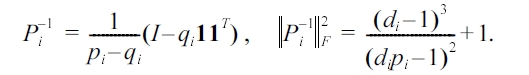
LEMMA 4. Let Pi be the randomization matrix specified in(1). When pi ≠ 1/di , we have
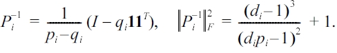
where 1 is the column vector, whose cells all equal 1.
PROOF. We can re-write Pi as follows:
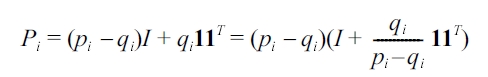
With
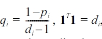
and the binomial inverse theorem[45], we can immediately get Pi-1, and ''Pi-1 F ''2 can be directly calculated from Pi-1 .
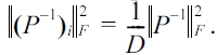
LEMMA 5. Let (P-1)i denote the i-th column (or row) of P-1.Then, for any i = 1, 2, . . . , D, we have
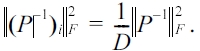
PROOF. With Lemma 4, we observe that every row (or column)of Pi-1has the same components, except for a change of order. Since P-1 = Pi-1 ? · · · ? Ps-1 , we can also conclude that all rows (or columns) of P-1 have the same components,except for a change of order. Therefore, for all i’s,
Next, we prove the main result. With Lemma 3, when the distance is the squared Euclidean distance, to minimize E[d(π? ,π)] is equivalent to minimize trace(Σ). With (2), we have
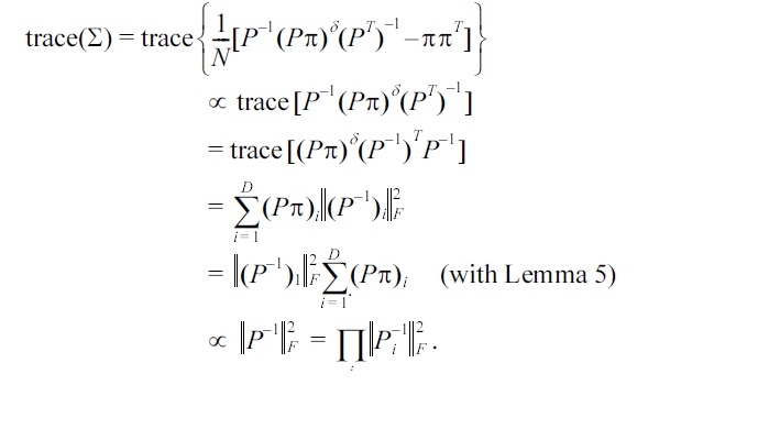
Notice that the constraint function is an increasing function of pi, the optimal solution must occur when the equality stands,and we have proved the result.