The geostationary earth orbit (GEO), located at about 35,786 km above the equator, is the orbit where the satellite orbit period is the same with the rotation cycle of the earth which was first calculated by Noordung (1929).Having the same orbital period with one sidereal day means that about 40 percent of the Earth surface can be observed for 24-hour by a single GEO satellite. This property is a great advantage for satellite communication and motivates more than 1,200 GEO satellites to launch since Syncom-2, was launched in 1963. Currently, about 400 geostationary satellites are operating (CelesTrack 2011). However, since the geostationary orbit is a limited space resource due to its features?a limit altitude and inclination,the allocation of GEO is managed by international organizations and the operation area of the GEO satellite is also limited to the range of 0.1° × 0.1°. Hence, for the efficient management of the limited space resource,it is important not only to track GEO satellites of one’s own country but also to surveil and track the satellites and space debris approaching the allocated domain.Air Force Research Laboratory Maui Optical and Supercomputing (AMOS) at Hawaii, USA and the Satellite Situational Awareness program of European Space Agency (ESA) are representative examples of GEO surveillance using an optical system (del Monte 2007).
The purpose of this study is to suggest the orbit determination strategy for the real-time surveillance of the space objects and space debris located near GEO. The system for the surveillance and tracking of GEO satellites requires rapid and accurate determination of the orbit of unidentified objects as well as continuous tracking and surveillance by efficient cataloging. In particular, choice of the rapid and stable orbit determination system is very important for an object near GEO since the observation time is limited for an optical observation based system.In this study, we employed the unscented Kalman filter (UKF) as the real-time orbit determination algorithm for rapid orbit propagation and orbit determination. We used the analytical dynamic model for the orbit propagation.The algorithm of the UKF proposed by Julier et al. (1995), enables to form the algorithm without linearization,different from the extended Kalman filter (EKF) that includes the linear approximation of nonlinear system, and thus has rigid characteristics of the nonlinear system. Roh et al. (2007) suggested that such an advantage of the UKF showed better performance in the satellite orbit determination than that of the EKF in the case where nonlinearity was intensified like the large initial error. On the other hand, the variation of mean orbital elements are slower than that of the osculating one, so it is easier way to use the mean elements for managing satellite database. However, the mean orbital elements is defined with the corresponding analytical orbit model, so satellite database using the mean orbital elements should be provide with the orbit model that used to generate the database. The osculating orbit can easily be recovered for short and long term through the accompanying orbit software by adding by secular, short and long term variation of the orbital elements. One of the representative analytical orbit propagation models for the geostationary orbit is the SDP4 model used by the North American Aerospace Defense Command (NORAD) to manage the satellite database so called Two Line Elements (TLE) (Hoots & Roehrich 1980). However, the SDP4 orbit model is too simple to use a latest high-resolution observation system. In this study, we used the analytical dynamic model developed by Lee et al. (1997). This model has been already applied to a time synchronization system based on a GEO satellite to which the EKF was applied, showing the orbit determination accuracy of several hundred meters (Yoon et al. 2004).
The main purpose of this study was to verify the availability of the orbit determination algorithm based on the analytical orbit dynamic model and the UKF as a geostationary orbit tracking and surveillance system. This article consists of following chapters: Chapter 2 explains the geostationary orbit determination system of this study; Chapters 3 and 4 describe the analytical dynamic model and the UKF that were applied to this study; Chapter 5 describes the result of the simulation experiment for various cases; and Chapter 6 made the conclusions.
An optical telescope is generally used for the observation of the surveillance and tracking of unidentified space objects and space debris located on the geostationary orbit because the altitude is very high as 35,800 km (Africano et al. 2004). One representative example is the 194charged coupled device (CCD) Debris Telescope (CDT) installed in AMOS, USA, of which diameter is 30 cm and viewing angle is about 1.7° × 1.7°, and it is generally used for the surveillance of space debris on the geostationary orbit (Africano et al. 2004). Flohrer et al. (2005) also reported that objects with the diameter of about 25 cm could be surveiled on the geostationary orbit using the ESA telescope with the diameter of 1 m and the viewing angle of 0.7° × 0.7°. In addition, the orbit can be precisely determined by applying appropriate dynamic model and estimation algorithm because the recent optical telescopes provide very precise observation data. Sabol & Culp (2001) showed that the orbit could be determined in the resolution of 10 meters using only the azimuth and elevation observation data of the Raven telescope with the observation precision of 1~2 arcsec.
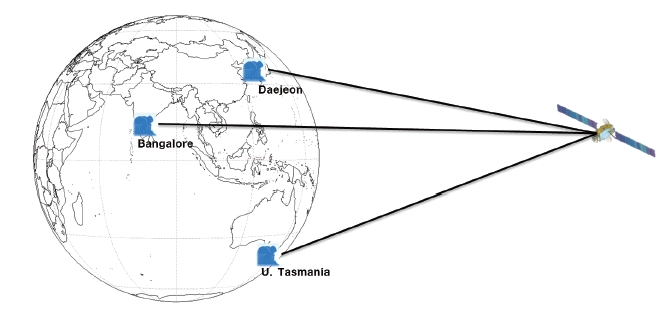
In this study, three ground stations in Korea, India and Australia were chosen as the tracking stations, forming a triangle in order to have the geometric distribution as wide as possible as shown in Fig. 1. Simulation experiments were also performed for the cases where the number of tracking stations was two and one. The specific locations of the individual observatories were set as shown in Table 1. The geostationary orbit has the advantages that there is almost no change in the azimuth and elevation because the GEO satellite looks stationary when viewed from the ground. However, the optical observation system has many limitations in the observation time due to the weather and eclipse. The main purpose of this study is to analyze the performance of the orbit determination algorithm suggested in this study. For this, the various tests were performed assuming that observation is possible for a certain period of time each day.
[Table 1.] Geodetic locations of ground tracking stations.
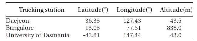
Geodetic locations of ground tracking stations.
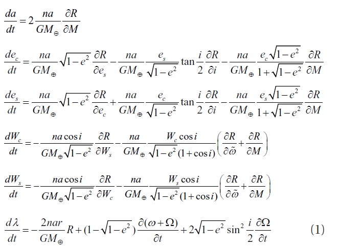
The orbit propagation model for the GEO satellite using the analytical method refers to the method to calculate the orbit elements at arbitrary time through the series expansion of the Lagrangian equation solution for the orbit elements (Lee et al. 1997). Since the eccentricity and the orbit inclination angle approach zero in the orbit propagation equation applied in this study, we used the equinoctial orbital elements,
where
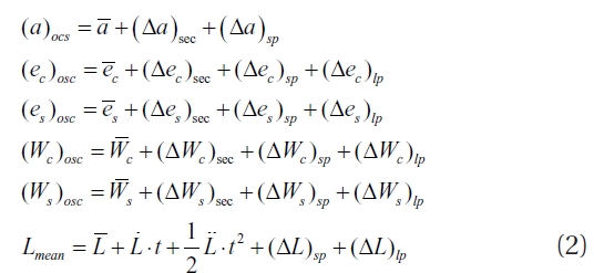
where
State variables should be carefully chosen to apply the analytical orbital propagation model to the real-time orbit determination algorithm. The reason was that, if osculating orbital elements were chosen as the state variables, the conversion of the osculating orbital elements to the mean orbital elements would be frequently required in the orbit propagation procedure and thereby not only the calculation speed but also the filtering performance would be decreased (Daum 2005). So, in this study, the orbital elements containing only the secular variation were chosen as the state variables. Moreover, the choice of the mean orbital elements as the state variables provides the advantage of management that the orbit determination result can be directly cataloged as in the case of TLE of NORAD.
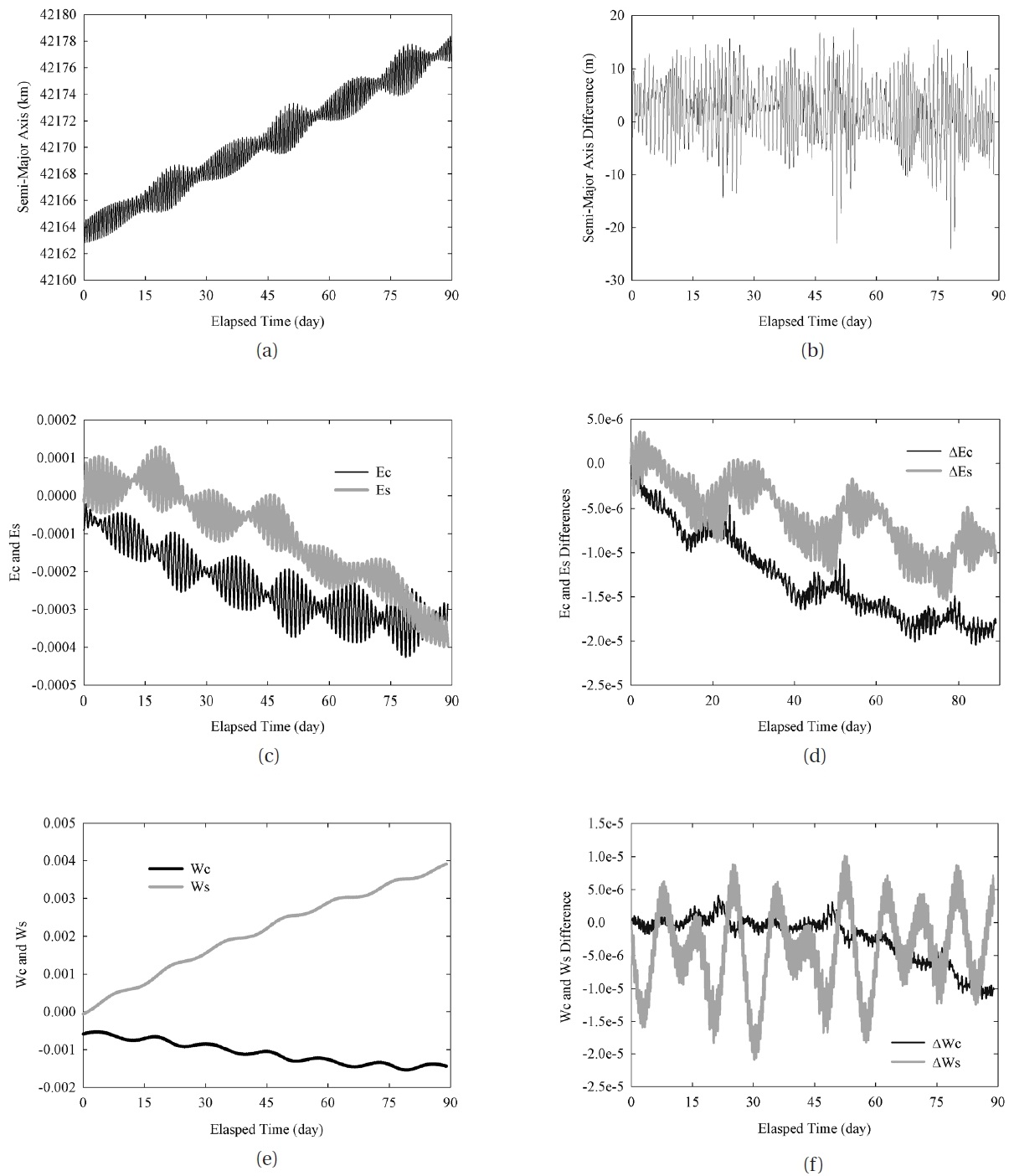
To verify the accuracy of the analytical orbit propagation model applied to this study, we compared the result with the orbit calculated by the high-precision orbit propagator (HPOP) module of satellite tool kit, a high-resolution numerical orbit propagation model (Analytical Graphics 1998). In HPOP, the 7(8)th order of Runge-Kutta integration method was used and the EGM96 gravity model up to 36 × 36 coefficients, the perturbation by the solar radiation pressure, and the three-body perturbation by the sun and the moon. In addition, the perturbations by the solid earth tide, the ocean tide and atmospheric resistance as well as the three-body perturbation by the major planets of the solar system were also included in the model to simulate as closely as possible to the actual state, although these perturbations are not included generally in the geostationary orbit model because of the little effect. Fig. 2 shows the difference between the orbit propagation for 90 days (epoch: 2005-5-7 12 h) by the analytical orbit model (left column) and the orbit propagation of the same initial orbit by HPOP (right column). Table 2 is the initial orbitals elements used in here. The comparison of the result with that by HPOP
[Table 2.] Initial epoch and orbital elements used for the truth orbit simulation.
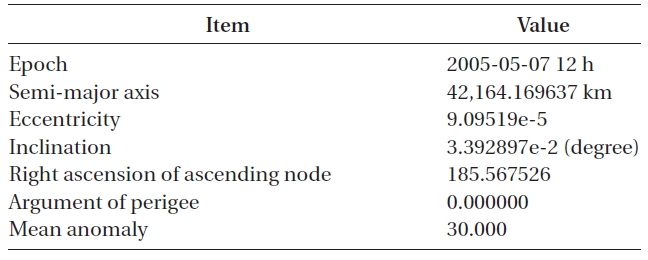
Initial epoch and orbital elements used for the truth orbit simulation.
showed that the error in the semi-major axis was about 20 m after the orbit propagation for 90 days and the error in other elements was about 2 × 10⁻⁵, which was similar to the result by Lee et al. (1997). The system noise level of the analytical orbit propagation model set as 1 m (1σ)
for the semi-major axis and 1 × 10⁻⁶ (1σ) for other orbital elements, considering the result described above and the short observation interval (one minute at most) set in this study. These values were applied to all the following simulation experiments.
The UKF has been used for studies in many application areas thanks to the advantage of using the nonlinear system without linearization. The UKF uses the statistical distribution of the state variables of the nonlinear equation, applying the state variables to the nonlinear system by sampling a number of state variables around the reference state variables called ‘sigma-point.’ Roh et al. (2007) showed that the UKF is better than the EKF in terms of the convergence speed, precision and robustness in the orbit determination based on the geomagnetic field observation.On the other hand, the UKF requires long computing time in most cases when numerical integration is used because orbit propagation should be performed for a great number of ‘sigma-points’ (Roh et al. 2007). However,the use of an analytical dynamic model, as in our study, may cancel off this drawback.
In general, the estimation algorithm begins with the definition of the system and the observation models as follows:
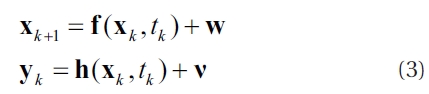
where X denotes the state vector, which is the mean equinoctial orbital elements, y the observation variables consisting of the azimuth and the elevation, and W and ν the system and observation noises, respectively. As mentioned in Chapter 2, the system function, f, includes only the secular variation and the long-period and short-period variations are used only when calculating the osculating orbit. The algorithm of the UKF is briefly described as follows:
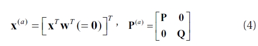
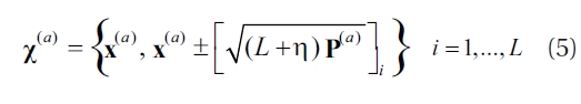
where P and Q denote the state vector and the covariance of the system noise vector, respectively,
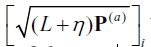
the
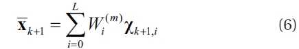
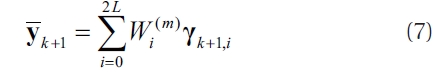
The state vector is calculated using the propagated sigma-points, χκ + 1 that are achieved by propagating the sigma-points calculated by Eq. (3). The observation vector is also calculated using the Eq. (3) with the state vector γκ + 1.
Additionally, the covariance and the cross covariance of the propagated state and observation vectors are calculated as follows:
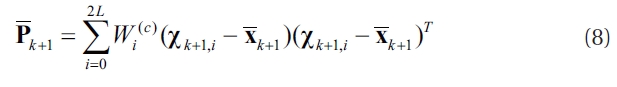
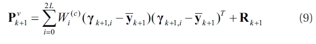
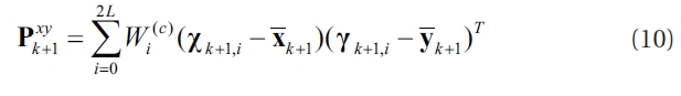
where the weights,
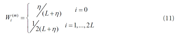
Here, the optimal value for β is known to be 2 for a Gaussian distribution (Wan & van der Merwe 2001). The update of the propagated state variables and the covariance is performed by the same equations of the EKF as follows:
where y
Whereas the UKF has the advantage that the nonlinear orbit propagation model can be used without linearization,it has the drawback that a total of 25 (= 2
The greatest drawback of the geostationary determination method based on an optical system is the limited observation time span. In particular, the orbit determination of unidentified GEO satellites or space debris lacking the initial orbital elements begins with a relatively large initial error. Thus, the orbit determination should be performed so that the orbit determination algorithm is not diverged and the tracking can be followed even at the next observable time, which is about one day later. For example, the telescope of 1 m diameter, which is used by ESA for the space object surveillance, has the viewing angle of about 0.7 degree, which corresponds to the error of about 500 km on the geostationary orbit. Therefore, the observation is possible when the orbital error after propagating the estimated orbit for about 24 hours is within 500 km.
This chapter describes the simulation experiments performed for various cases to verify the geostationary orbit tracking and surveillance realized in this study. The truth orbit for the simulation experiments was calculated by HPOP as described in Chapter 2. With respect to the azimuth and elevation calculated for the ground stations in Table 1, different white noises were applied for the simulation experiments. The truth orbit was generated with reference to the same reckoning date of July 1, 2005, as in the test results in the previous chapter. The orbit, the longitude 116° geostationary orbit, was set to have the same mass and cross-sectional area, which are 700 kg and 21.0 m2, respectively. Following sections are the orbit determination results for the various level of initial error and measurement noise, the different time interval of the measurements, and the different number of ground station.
5.1 Effect of the Initial Error
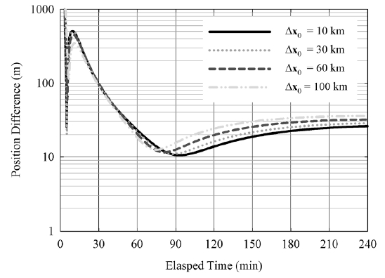
In cases of the GEO satellites or space debris of which initial orbit information is unknown, the possibility of continuous tracking is determined by how rapidly and precisely the estimation filter can converge from the relatively large initial error. In this study, we performed the orbit determination applying the error of 10 km, 30 km, 60 km and 100 km to the initial position vector of the truth orbit. Thus, the positional error of the maximum 170 km was taken into account. For the experiment, we assumed that there were three observatories shown in Table 1, the observation time interval was 5 seconds, and the observation precision was 5 arcsec. The tests results are summarized in Fig. 3. Even when the maximum observation precision is assumed to be 60 arcsec, the maximum initial error does exceed 100 km because the distance error of 60 arcsec is just about tens of kilometers. If only angular measurements are used, more than 100 km of the initial orbit error is meaningless because the satellite is out of the viewing angle of the optical telescope. However, as shown in Fig. 3, the convergence was made to the level of 100 m when the simulation was continued for about 30 minutes.
5.2 Effect of the Observation Time Interval
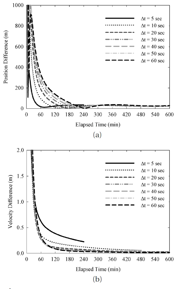
When performing optical observation of the geostationary orbit, the observation time should include the CCD exposure time and the time taken to generate the angle information through the data processing. In this test, we examined the orbit determination performance varying the observation time interval from 5 seconds to the maximum 60 seconds. The number of ground observatories was three and the precision of the observation value was 5 arcsec, just as in the previous test regarding the initial error. The initial error of 100 km was applied for each axis, so the filtering was started with the initial positional error of about 170 km. Fig. 5 shows the test
result of different observation time intervals. Each case had the same number of observation data, i.e., a total of 2,880 observation times were processed. In other words, 720 data per hour were processed when the observation time interval was 5 seconds (four hours of observation
time), and 60 data per hour were processed when the observation time interval was 60 seconds (ten hours of observation time). Table 3 summarized the mean orbital error for 30 minutes after one hour of data processing for each case. In all the cases, the orbital error was converged to less than 300 m after one hour of data processing. As Fig. 4 shows, the orbital determination precision was converged to the similar level after processing the same number of observation data. The orbit error after 24 hours following one hour of data processing in a 60 second interval was about 7.9 km, indicating that continuous tracking was possible. On the other hand, the velocity element was converged more rapidly as the observation time interval was longer, as shown in Fig. 4. The reason why the velocity element showed different trend is that the observation information is biased to the positional element. In other words, the velocity element is more precise at the same error level as the observation time interval was longer. Moreover, as the positional element is rapidly converged, the covariance of the velocity element is also reduced, resulting in slow convergence of the velocity element.
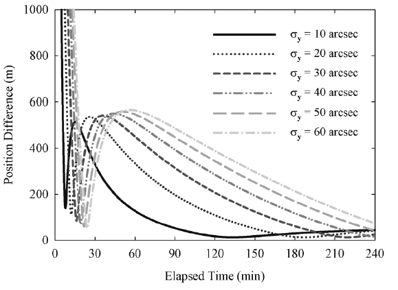
5.3 Effect of the Observation Error Level
In this test, we analyzed the orbit determination performance depending on the observation precision of the optical system. The observation error was simulated as the white noise for the azimuth and elevation individually.The orbit determination was performed for the error level ranging from 10 arcsec (1σ) to the maximum 60 arcsec(1σ) to verify the strategy of this study for various optical telescopes. The number of the ground observatories and the observation time interval were set to be 3 and 5 seconds, respectively. The initial error of 100 km was applied to the angular axis. Fig. 5 shows the orbit determination result depending on the observation error level.
[Table 3.] Results for the different measurement interval (during 30 minutes after 1-hour).
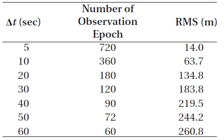
Results for the different measurement interval (during 30 minutes after 1-hour).
Even though the convergence speed and the orbit determination precision were varied by the observation error, the root mean square orbit error after about one hour of processing was converged to 600 m in all the cases. Considering that the observation precision of the general geostationary tracking and surveillance telescopes is less than 10 arcsec, the tracking and surveillance can be carried out well through the algorithm applied in this study.
5.4 Effect of the Number of Ground Observatories
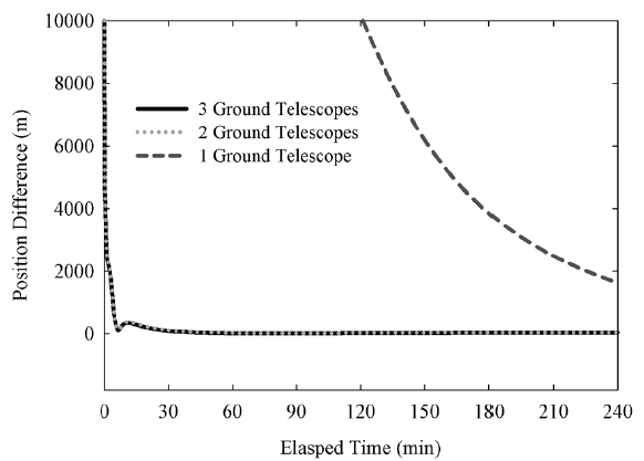
In this section, we analyzed the orbit determination result depending on the number of ground observatories. As shown in Fig. 1, the orbit determination was performed with the ground observatories in a triangular form in all the previous tests. It was because it is ideal to arrange the ground stations to have the geometric distribution as wide as possible because the geostationary orbit has the high altitude of 35,800 km and it looks as if stationary when viewed from the ground. Fig. 6 shows the orbit determination results for one station in Daejeon, two in Daejeon and Bangalore, and three additionally at Tasmania University in Australia. As Fig. 6 shows, there was almost no difference between the cases where the number of ground observatories was 2 and 3. However, the convergence speed was much lower when only one ground observatory was included: the orbit error was converged to less than 10 km after about two hours.
In this chapter, we performed orbit determination applying different initial error levels, observation precision levels, observation time intervals and different number of ground observatories in order to analyze the performance of the orbit determination system for the geostationary orbit satellites based on analytical orbital dynamics and UKF. The simulation test results showed that
the algorithm suggested in this study is available for the tracking and surveillance of geostationary orbit satellites.
In this study, we developed the orbit determination algorithm for geostationary orbit satellites based on optical observation system to track and surveil geostationary orbit satellites. Tests were carried out for various cases to verify the availability and validity of the suggested strategy. Firstly, we employed the UKF as the orbit determination algorithm and the analytical orbit propagation equations to improve the calculation speed of the UKF. We made the space object tracking and surveillance database management easier by setting the mean orbital elements as the estimation vectors for the orbit determination.
The tests performed in this study assumed an optical observation system. The orbit determination performance was focused on not only the final orbit determination precision but also continuous tracking possibility. In the test with the initial error greater than 100 km, the convergence was rapidly made to about several tens of meters after one hour, assuming that the observation was performed at three ground stations with the angular resolution of 5 arcsec and the observation time period of 5 seconds. Considering that the about 1° of viewing angle corresponds to about 700 km on the geostationary orbit, tracking can be continuously performed even after one day. When the initial error was small, the orbit was stably determined to about 10 m accuracy after one hour of orbit determination process. On the other hand, there was almost no difference between the cases where the number of ground observatories was 2 and 3. However, when there was only one ground observatory, a considerably many number of continuous observation data were required for the convergence speed and precision because of the geometrical limitation. The results in this study used the simulated orbit and observation values. In the future, tests may need to be performed considering the constraints such as weather and eclipses as well as the precision of optical system in order to apply an actual system.
The orbit determination algorithm for the geostationary orbit tracking and surveillance developed in this study is useful not only to protect the geostationary satellites but also to protect a GEO area assigned to a country from the threat of unidentified space objects in the future.