Satellite navigation system plays an increasing role in modern society. Various satellite navigation systems are in operation and being currently developed including global positioning system (GPS), global navigation satellite system (GLONASS), and Galileo. Thus, there is an increasing need for the research and development in various areas such as signal generation, signal reception, precise positioning, high-precision geodesy and survey in relation to the individual satellite navigation systems.The global navigation satellite system (GNSS) simulator has drawn more and more attention in recent years due to it can conduct these studies efficiently regardless of surrounding condition (Dong et al. 2004).
An actual GNSS signal is affected by various errors before arriving at the antenna after being transmitted from a satellite. Hence, modeling of the GNSS error factors is required to generate the signals similar to the actual GNSS signals using the GNSS simulator. Among various kinds of error factors, the signal delay by the ionosphere is the greatest after the elimination of selective availability and it must be included in the modeling to reflect the effect.
One of the modeling methods for ionospheric delay is the ionosphere-free combination using dual frequency measurements (Hofmann-Wellenhof et al. 2007). The ionosphere-free combination is the method by which the geodetic results free from the ionospheric delay can be obtained by removing the ionospheric delay term in the linear combination of the dual frequency code pseudorange observables. However, since the dual frequency receiver is relatively expensive, the method cannot be applied to single frequency receivers that are frequently used by casual users. Thus, for single frequency receivers,the ionospheric models are employed to estimate the ionospheric delay and one representative model is the Klobuchar model. The Klobuchar model is the most widely used one because the structure is simple and the calculation is convenient (Yuan et al. 2008). In order to use the Klobuchar model, eight Klobuchar coefficients, αn, βn (
As the previous study related to this, Lee et al. (2010) collected the Klobuchar coefficients included in the navigation messages from 2006 through 2008 and developed the Klobuchar coefficient generating model by analyzing the tendency of the individual coefficients over time. However, the model developed by Lee et al. (2010) is limited in the accuracy of the Klobuchar coefficients because it consists of simple cosine functions and linear functions.
Therefore, in this study, a Fourier series-type model was developed by analyzing the tendency of the Klobuchar coefficients provided for three years between 2006 and 2008 to elevate the accuracy of the Klobuchar coefficients estimation. The Fourier series is a mathematical technique by which periodic functions are decomposed into the weights of trigonometrical functions. The Klobuchar coefficients generating model developed in this study was defined as Fourier Klobuchar model (FOKM) and the Klobuchar coefficients generated by using FOKM were defined as FOKM coefficients. Moreover, we defined the model developed by Lee et al. (2010) as the modified model (MODL). Using FOKM and MODL models, we derived the total electron content (TEC) and compared it with the result of broadcast (BRDC) to verify the improved estimation accuracy.
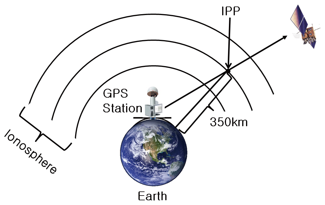
In the Klobuchar model, the GPS ionospheric error is estimated by calculating the TEC between the GPS satellite and the GPS receiver, and the total ionospheric error can be eliminated up to approximately 50 to 60% depending on the solar activity or the region. (Klobuchar 1987, Komjathy 1997). To use the Klobuchar model, it is assumed that free electrons are concentrated on an imaginary single layer of which thickness is zero at the 350 km altitude, as shown in Fig. 1, the TEC is at the peak at the local time (LT) of 2 o’clock p.m., and the TEC is constant as 9.24 TEC unit (TECU) between 22:00 and 06:00 (Klobuchar 1987). One TECU means that 1016 free electrons exist in the area of 1 m2. When converted to the distance error, 1 TECU corresponds to 0.163 m (Hofmann-Wellenhof et al. 2007).
The Klobuchar model employs geomagnetic latitude on ionosphere pierce point (IPP). As shown in Fig. 1, IPP is defined as the point where the line of sight that connects the GPS satellite to the signal reception point meets the single layer. Since the change of TEC at IPP is affected by seasons and the geomagnetic field and closely related with the sunspot activity, it is varied following the solar activity in the period of 11 years.
In order to use the Klobuchar model, the Klobuchar coefficients, αn and βn, are required and they are generated by two criteria. The first criterion is the observation date. The GPS Master Control Station divided one year into 37 intervals and assigned the Klobuchar coefficients group corresponding to each interval. The second criterion is the mean of the solar flux for the previous five days including the corresponding day. The solar flux is classified into 10 grades and the Klobuchar coefficients groups are designated for the individual grades. The GPS Master Control Station select αn and βn considering the observation date and the solar flux value and provide them through the satellite navigation message (Seo 1994, Ovstedal 2002).
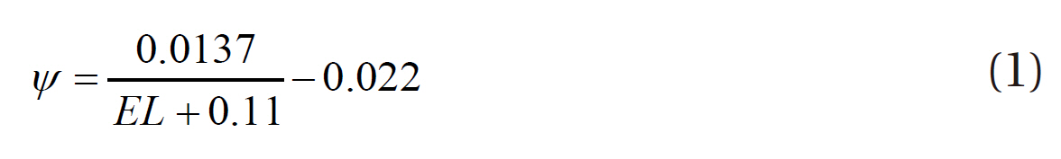
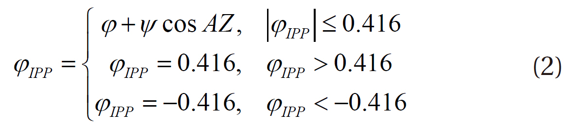
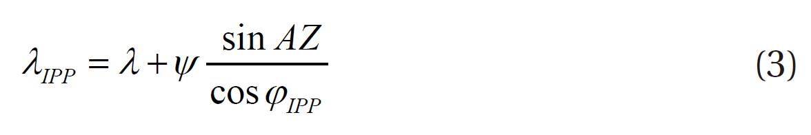
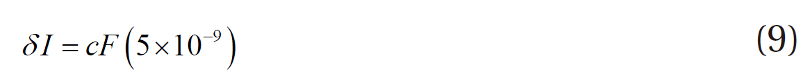
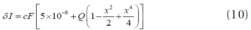
The calculation of the ionospheric delay using the Klobuchar model follows the procedures from Eq. (1) to Eq. (10). The detailed explanation on the equations can be found in Klobuchar (1987). In Eqs. (1) and (2), ψ denotes the Earth-centered angle, EL the GPS satellite elevation angle, φ the geodetic latitude, AZ the GPS satellite azimuth, and ΦIPP the subionospheric latitude. After calculating the subionospheric latitude, the subionospheric latitude, λIPP, is calculated using Eq. (3) where λ denotes the geodetic longitude. If the satellite elevation angle is 90°, the IPP is located in the vertical direction of the reception point and thus the vertical TEC (VTEC) is calculated.
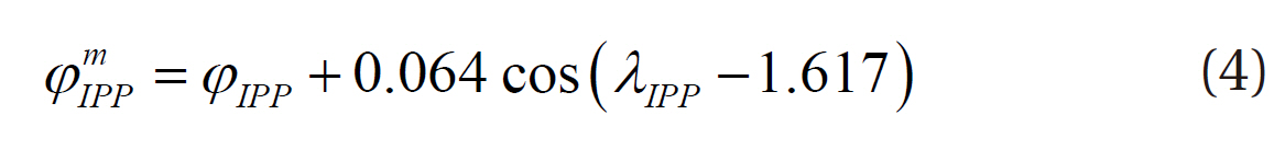
Next, the geo-magnetic latitude, ΦmIPP, is calculated using Eq. (4). Then, the GPS time (sec),
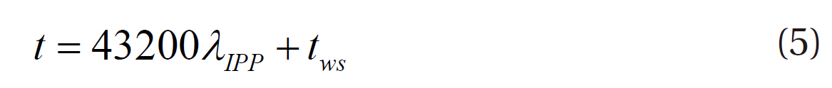
For the next, the Klobuchar coefficients, αn and βn, are substituted into Eqs. (6) and (7) to calculate the conversion factors
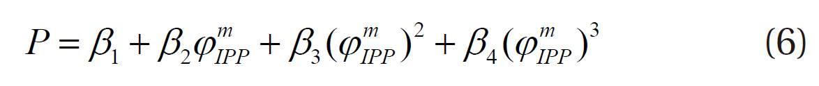

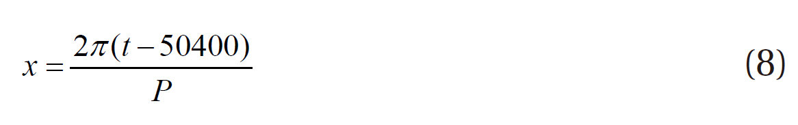
Finally, the P calculated by using Eq. (6) is substituted into Eq. (8) to calculate
3. DEVELOPMENT OF KLOBUCHAR COEFFICIENTS GENERATION MODEL USING FOURIER SERIES
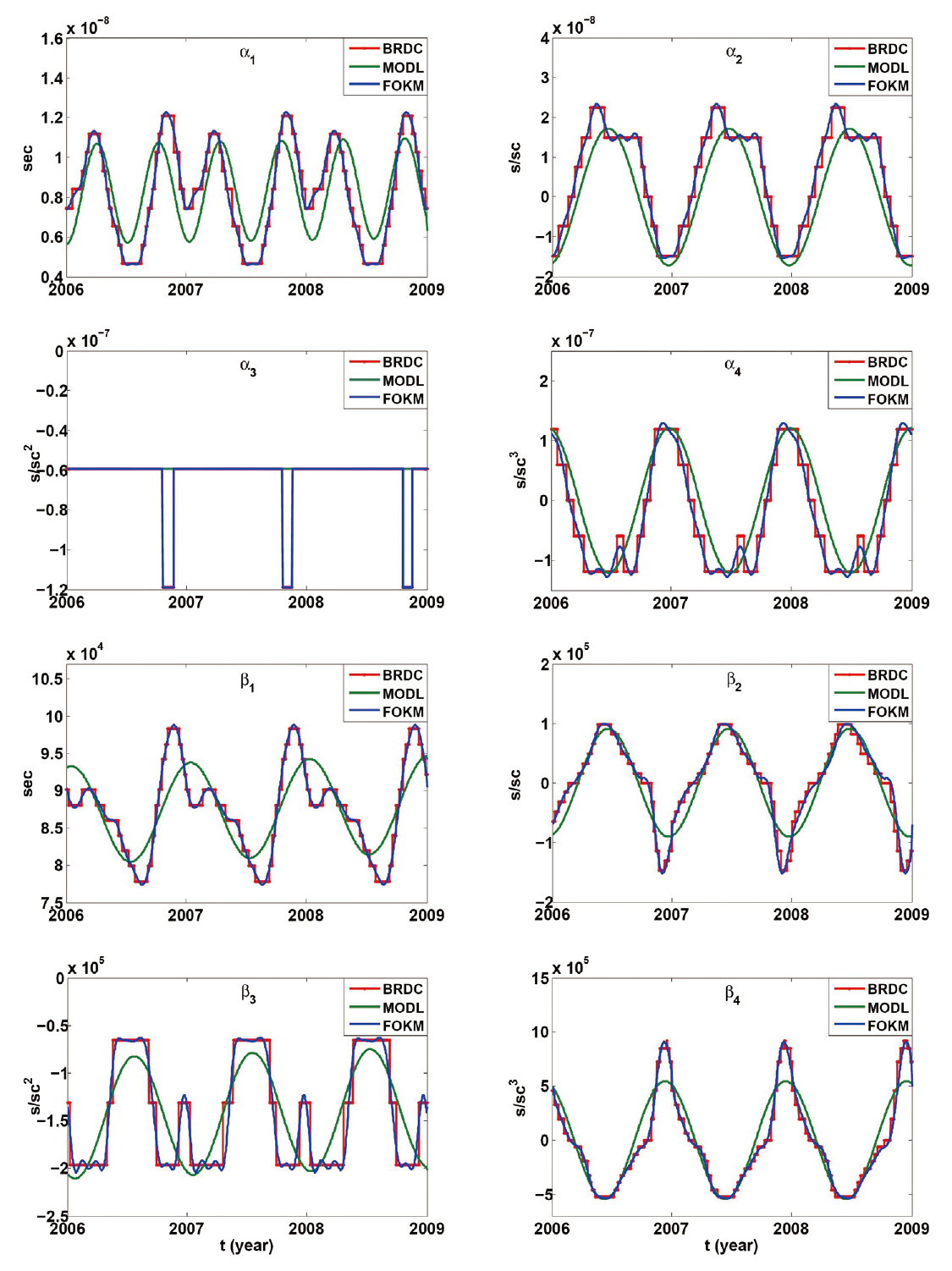
In this study, we employed BRDC, the navigation message provided by International GNSS Service (IGS), to develop FOKM. BRDC is the navigation message that contains the two-hour interval BRDC ephemeris of all the GPS satellites that are currently in operation and it includes the Klobuchar coefficients, αn and βn, in the header part. Since BRDC is generated in one-day interval and can be provided from the IGS website without charge, it is very convenient to analyze the change in the BRDC coefficients according to the lapse of days. In this study, after collecting the Klobuchar coefficients contained in BRDC from 2006 through 2008, the tendency over time was analyzed for each of the coefficients to develop the model in the form of Fourier series. The orders of individual Fourier series, except α3, were selected as the orders that generate the least RMS error between the FOKM coefficients and BRDC coefficients. As a result, the eighth order was selected for α1, α2, β1 and β3, the seventh order for β2, and the sixth order for α4 and β4. The value of α3 was shown to be -5.96 × 10⁻⁸s/sc2 in most of the period in a year, and it was -11.92 × 10⁻⁸ s/sc2 only in the period from the middle of October through the middle of November. Thus, α3 was not modeled not in the form of Fourier series but in the form of a constant for which a conditional sentence is given for the date.
Fig. 2 shows the BRDC coefficient (blue line), the FOKM coefficient (red line) and the MODL coefficient (green line) developed by Lee et al. (2010). The horizontal axis represents the observation time in years, while the vertical axis represents the individual units of the Klobuchar coefficients. In the units for the vertical axis, s denotes second and sc denotes semi-circle. As can be known from Fig. 2, the BRDC coefficient is repeated in one-year cycle, and the FOKM and MODL coefficients also show the cycle of one year, accordingly. It can be verified with naked eyes that the MODL coefficient follow the overall tendency of the BRDC coefficient but not as precisely as the FOKM coefficient.
To assess the accuracy of FOKM developed in this study, the correlation coefficients of FOKM and MODL with respect to BRDC were determined, as shown in Table 1. The result shows that the correlation coefficients of FOKM were higher than those of MODL for all the coefficients. In particular, all of the correlation coefficients between FOKM and BRDC were equal to or higher than 0.97. In the case of α3, the correlation coefficient between BRDC and FOKM was not 1 because the period when the value was found to be -11.92 × 10⁻⁸ s/sc2 was not identical every year.
[Table 1.] Correlation coefficients of MODL and FOKM based on BRDC (Lee et al. 2010).
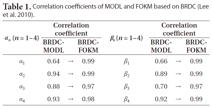
Correlation coefficients of MODL and FOKM based on BRDC (Lee et al. 2010).
4. VERIFICATION OF THE ACCURACY OF FOKM
To verify the accuracy of FOKM generated by using the BRDC coefficients between 2006 and 2008, the VTEC above the Daejeon (DAEJ) GPS station was calculated from January 1 to December 31 in 2009. For this, the observation time which is the input data of the Klobuchar model was fixed to analyze the effect of only the FOKM coefficients and BRDC coefficients. Additionally, the elevation between the GPS satellite and the DAEJ, which is
required for the Klobuchar model, was fixed at 90° to calculate the VTEC above station regardless of the position of the satellite. Then, we compared the VTEC calculated by inputting the FOKM coefficients and those calculated by inputting the BRDC and MODL coefficients.
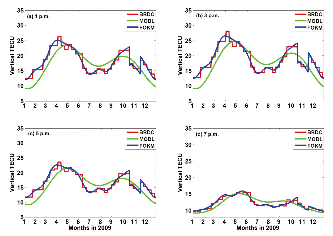
Fig. 3 shows the VTEC of the three Klobuchar models in one-day interval calculated by using the two-hour interval of observation time, that is, the observation time fixed at 1, 3, 5 and 7 o’clock p.m. In Fig. 3, the red, green, and blue lines represent the results of BRDC, MODL, and FOKM, respectively. The VTEC from the individual models were varied depending on the observation times, the highest at 3 p.m. and the lowest at 7 p.m. This is because, in general, the solar activity is at its peak in the time around 2 and 3 o’clock p.m. Individual comparison of MODL and FOKM with respect to BRDC indicated that the FOKM results showed the tendency similar to that of the BRDC results at all the observation times. The VTEC of FOKM was drastically changed in the period from the middle of October through the middle of November because α3 was modeled with the value of -11.92 × 10⁻⁸ s/sc2 for that period.
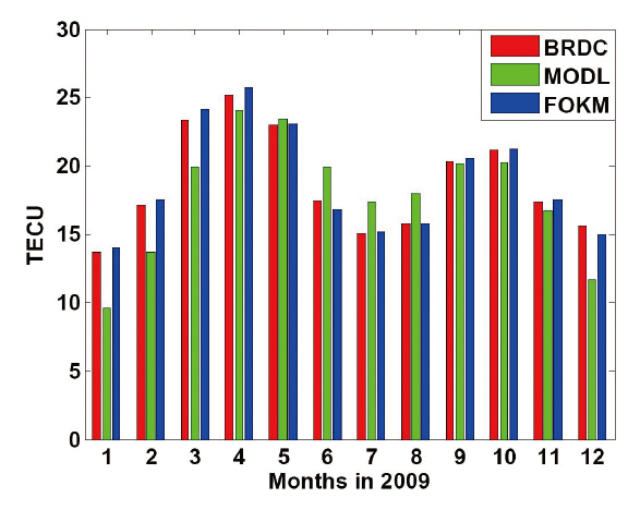
Using the result shown in Fig. 3, we compared the monthly mean VTEC of the three models as well as the RMS difference among the models. Fig. 4 shows the monthly mean VTEC of the three models calculated for the 3 p.m. epoch. The observation time of 3 p.m.was selected because the VTEC difference among the models was the most distinguishable at that time. Fig. 4 shows that the VTEC was the highest in spring, March and April, which is because the ionosphere is active around the spring equinox (Lee et al. 1995). The characteristics of the individual months show that the VTEC of BRDC and FOKM was higher than that of MODL from January through April and from September through December, and the difference was the maximum 4.3 TECU in January and the minimum 0.2 TECU in September. On the contrary, the result of MODL was higher than those of BRDC
or FOKM in summer, from May through August, and the difference was the maximum 2.4 TECU in June and the minimum 0.4 TECU in May. This is because MODL did not catch up with the tendency of BRDC and thus it was modeled relatively high in the period from May through August while it was modeled as lower than BRDC in the rest of the period.
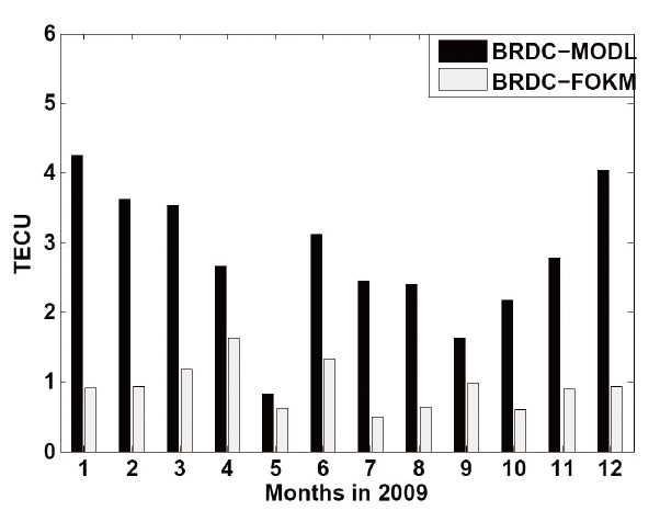
Fig. 5 shows the root mean square (RMS) difference of FOKM and MODL with respect to BRDC at each month, based on the result in Fig. 4. The result showed that the RMS difference between BRDC and FOKM was smaller than that between BRDC and MODL all over the analyzed period. The maximum RMS difference between BRDC and MODL was 4.3 TECU in January, and the minimum was 0.8 TECU in May. On the other hand, the maximum RMS difference between BRDC and FOKM was 1.6 TECU in April, and the minimum was 0.5 TECU in July. The deviation of the RMS difference was also smaller in FOKM than in MODL. Therefore, it is assumed that FOKM developed in this study is more appropriate than the MODL in performing the ionospheric delay modeling using a GNSS simulator.
In this study, we developed FOKM in the form of Fourier series by analyzing the time-dependent tendency of the BRDC coefficients provided through the navigation message for the three years from 2006 through 2008. All the correlation coefficients between the BRDC coefficients and FOKM coefficients were equal to or higher than 0.97. To determine the accuracy of FOKM developed in this study, VTEC was calculated by inputting the BRDC, FOKM and MODL coefficients individually to the Klobuchar model and the results were compared. The result showed that the maximum RMS error between the individual VTEC calculated by using the BRDC and MODL models was 4.3 TECU, which was larger by 2.7 TECU than the maximum RMS error between the BRDC and FOKM models, 1.6 TECU. Because the true VTEC value was assumed to be from BRDC, we calculated that FOKM developed in this study is more appropriate than the MODL in modeling the ionospheric delay error if the GNSS signals are generated using a simulator. However, because the BRDC coefficients only in the period of the solar minimum were taken into account for the model developed in this study, future studies should use the BRDC coefficients of 11 years including both the solar maximum and minimum periods to develop the ionospheric error environment model for the GNSS simulators.