The shape of the magnetosphere is changed by many factors such as the solar wind conditions, interplanetary magnetic field and various electric currents within the magnetosphere. Since the spatio-temporal variability of the magnetosphere is closely related with the changes in the magnetic field within the magnetosphere, many studies have been conducted from the past about the correlations of the solar wind, interplanetary magnetic field factors, and various electric currents within the magnetosphere with the changes in the magnetic field inside the magnetosphere.

Kokubun (1983) conducted a statistical study on the magnetic local time (MLT) dependence of the sudden storm commencement (SSC) that takes place when interplanetary shock passes by the magnetosphere. Using the geosynchronous magnetic field data, Kokubun suggested that day-night local time asymmetry appears during SSC:the effect of the magnetopause current is outstanding in the time period around the dayside, while the effect of magnetotail current is outstanding in the time period around the nightside.

McComas et al. (1993) conducted a study using the geosynchronous plasma data and discovered that geosynchronous satellites frequently observed the magnetosheath plasma in the morning sector (09:00 to 10:00 MLT). Such observations imply that the geosynchronous satellites pass through the magnetopause more often when they are in the morning sector than in the afternoon sector. They suggested that the cause of the morning-afternoon asymmetry of magnetopause crossing be the asymmetric erosion of the magnetic field in the morning sector or asymmetric ring current. Additionally, Dmitriev et al. (2004) studied the morning-afternoon asymmetry of magnetopause crossing using more geosynchronous magnetopause crossing data. Dmitriev et al. mentioned that geosynchronous magnetopause crossing can take place even at a relatively smaller solar wind dynamic pressure (5-6 nPa) in the morning sector (about 10:00 MLT) as the southward component of the interplanetary magnetic field is stronger. This indicates that peak of the magnetopause is placed in the morning sector, not at the local noon.

In the statistical analysis of the recent geosynchronous magnetic field data by Borovsky & Denton (2010), it was verified that the peak of the average geosynchronous magnetic field data in each season is laid not at the local noon but in the morning sector. Although Borovsky & Denton (2010) did not mentioned about the asymmetry of the magnetic field, the result indicates that the morning-afternoon magnetic field strength asymmetry may take place even when the magnetosphere is under the quiet time since the seasonal averages of the geosynchronous magnetic field can represent the values at the time when the magnetosphere is not perturbed.

Kim et al. (2007) statistically observed that the geosynchronous magnetic field is more compressed in the morning sector than in the afternoon sector during SSC. Motivated by this, we investigated in this study whether or not the morning (06:00-12:00 MLT)-afternoon (12:00-18:00 MLT) asymmetry of the geosynchronous magnetic field is found in the geomagnetically quiet time where the magnetosphere is not greatly perturbed and what factors affect the morning-afternoon asymmetry. Rufenach et al. (1992) suggested that the solar wind dynamic pressure affects greatly the H component of the geosynchronous magnetic field in the geomagnetically quiet time. Therefore, in this study, we performed statistical analysis of magnetic field data and investigated the causes of the asymmetry concerning the correlation of the dynamic pressure at the quiet time and the solar wind dynamic pressure, for each interval, with the morning-afternoon asymmetry of the geosynchronous magnetic fields in the dayside (06:00-18:00 MLT). Section 2 explains the data selected for this study and Section 3 describes the morning-afternoon asymmetry of the geosynchronous magnetic fields using the observed data. In Section 4, the statistical analysis about the asymmetry is stated. Section 5 is devoted to the comparison the results with the geomagnetic field model and Section 6 is the discussion of this study.

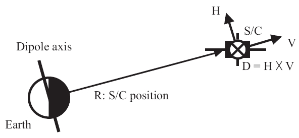
To investigate the change of the dayside (06:00-18:00 MLT) magnetic fields in the geosynchronous magnetosphere, we used magnetic field data from the Geostationary Operational Environmental Satellites (GOES) located near the magnetic equator (MLAT ~4°) among the GOES satellites operated for nine years (from February 1998 to January 2007). Within the period, the GOES satellite observation data are missing between August 1998 to March 1999, and between June 2005 and August 2005. We used the 1-min time resolution GOES satellite position data and magnetic field data provided by U.S. National Aeronautics and Space Administration (NASA) (http://cdaweb.gsfc.nasa.gov/). The changes of geosynchronous magnetic field data referring to the Earth’s dipole axis were examined more clearly by analyzing the geosynchronous magnetic field data after converting the geocentric solar magnetospheric coordinates data provided by NASA to the dipole VDH coordinates. Fig. 1 shows the VDH coordinates. The H component is defined as the component that is antiparallel to the direction of the Earth’s dipole axis, the V component as the component parallel to the magnetic equator directing outwards, and the D component as the H × V component. Since the strength of the H component magnetic fields can be replaced by the total magnetic field strength in the

day sector geosynchronous orbit, we investigated in this study the morning-afternoon asymmetry of the geosynchronous magnetic fields using only the H component. Because the changes of the geosynchronous magnetic field are correlated with the degree of magnetosphere perturbation by the solar wind, we used the Kp index that denotes the degree of the geomagnetosphere perturbation and the solar wind dynamic pressure data at the Advanced Composition Explorer (ACE) satellite. The solar wind data at the ACE satellite were the 1-min resolution data that were time-shifted by the bow shock nose point provided by NASA (http://omniweb.gsfc.nasa.gov/). The Kp index was provided by Kyoto University (http://wdc.kugi.kyoto-u.ac.jp/index.html).

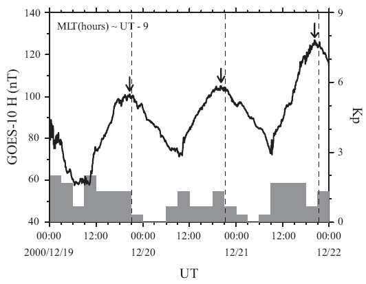
We defined the geomagnetically quiet time as the time when the Kp index is less than 3 (Kp < 3). The morning-afternoon asymmetry of the geosynchronous magnetic field was investigated by using the GOES satellite data under the geomagnetically quiet time. Fig. 2 shows the Kp index and H-component magnetic field during the three days from December 19 to 21 in 2000. The Kp index is shown as gray bars and the magnetic field as a black line. The local noon is expressed as the vertical dotted line. The Kp index in the three days corresponded to the

geomagnetically quiet time. During this period, the geosynchronous magnetic fields were larger in the morning sector than in the afternoon sector. In addition, it was observed that the peaks of the magnetic field strength were in the morning region with the local noon at the center (indicated by the arrows).

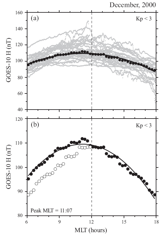
The gray dots in Fig. 3a represent the magnetic field observed for one month in December 2000, at the geosynchronous satellite, of which Kp index was lower than 3. The vertical dotted line indicates the local noon. To statistically investigate the morning-afternoon asymmetry of the geosynchronous magnetic field, the H-component the magnetic field data were divided into the 15-min MLT intervals and the medians of the intervals were expressed as black circles. The medians of the 15-min MLT intervals were used in order to examine if the aberration effect (atan[30/400] ~4° [about 15 minutes]) due to the

solar wind speed toward the Earth (~400 km/s) and the Earth’s orbital motion speed (~30 km/s) is related to the morning-afternoon asymmetry of the geosynchronous magnetic field. The black lines represent the second-order polynomial fitting curve of the medians and the error range was ±7.5 minutes.

To investigate the morning-afternoon asymmetry of the geosynchronous magnetic field in detail, the medians and its second-order polynomial fitting in December, 2000 were shown in Fig. 3b once again. The medians in the afternoon sector were flipped over with respect to the morning sector, having the local noon at the center, and marked as white circles. The peak of the second-order polynomial fitting was located on 11:07 MLT. Comparing the medians of the magnetic field data in the morning and in the afternoon, it was found that the magnetic fields in the morning sector were larger than those in the afternoon sector by 5~8 nT, approximately.

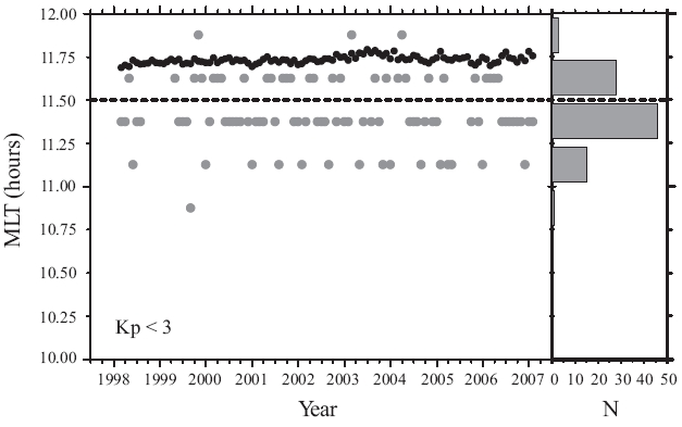
To examine whether or not the peak location of the geosynchronous magnetic field is because of the solar wind aberration effect, the solar wind data of the ACE satellite were statistically investigated. The peak locations of the geosynchronous magnetic field in each month during the observation period were calculated by the method in Fig. 3 and showed in Fig. 4 as gray circles. The black circles represent the locations of the magnetopause ob-

tained by using the aberration angle calculated on the basis of the solar wind speed data observed by the ACE satellite and the Earth’s orbital motion speed. Since the typical solar wind speed is 400~450 km/s, the obtained aberration angle was about 3.8-4.3° (corresponding to about 15 minutes). The histogram on the right shows the number of the peak location of the geosynchronous magnetic field. Considering the error range of ±7.5 minutes, about 30% of the total number of the peaks located at 11:37 MLT can be accounted for by the aberration effect (the region above the dotted line). On the contrary, since about 66% of the peaks are located between 11:07 and 11:22 MLT, the morning-afternoon asymmetry of the geosynchronous magnetic field may not be accounted for just by the aberration effect (the region below the dotted line).

Shue et al. (1998) mentioned the solar wind dynamic pressure as one of the factors that determine the changes in the shape and size of the magnetopause. Hence, we investigated the solar wind data of the ACE satellite to examine if the solar wind dynamic pressure is correlated with the morning-afternoon asymmetry of the geosynchronous magnetic field. The average of the solar wind dynamic pressure during the observation period of this study was about 2.2 nPa which was similar to the average solar wind dynamic pressure under the geomagnetically quiet time in the study of Tsyganenko & Sitnov (2005), 2 nPa. Based on this, we set the boundary value to 2 nPa of the solar wind dynamic pressure and analyzed the cases by considering the case with the solar wind dynamic pressure lower than that as the case with little solar wind effect and the case with the solar wind dynamic pressure at or higher than that as the case with great solar wind effect.

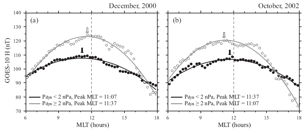
Fig. 5a shows the medians and the second polynomial fitting curve of the geosynchronous magnetic field data in December 2000, in the cases of the solar wind dynamic pressure lower than 2 nPa, and at or higher than 2 nPa. In the cases where the solar wind dynamic pressure was lower than 2 nPa, the peak of the polynomial fitting was located at 11:07 MLT which is the same with that of the polynomial fitting time obtained in the cases where the Kp index was smaller than 3 (indicated by a black arrow). In the cases where the solar wind dynamic pressure was at or higher than 2 nPa, the peak of the polynomial fitting inwas located at 11:37 MLT, moved toward the local noon (indicated by a white arrow).

To investigate if the peak of polynomial fitting is always moved toward the local noon region when the solar wind dynamic pressure is large, as in Fig. 5a, the medians and the peak of the polynomial fitting were showed in Fig. 5b for the cases when the solar wind dynamic pressure was lower than 2 nPa, and at or higher than 2 nPa, using the magnetic field data of the geosynchronous satellite in October 2002. In the case of October 2002, the peak of the polynomial fitting was located at 11:37 MLT when the solar wind dynamic pressure was lower than 2 nPa (indicated by a black arrow), while that was located at 11:07 MLT when the solar wind dynamic pressure was at or higher than 2 nPa (indicated by a white arrow). Thus, it could not be known how the peak of the geosynchronous magnetic field is correlated with the solar wind dynamic pressure based only on the data of December 2000 and October 2002.

However, one interesting point found in these two cases was that the peak locations were correlated with the magnetic field asymmetry between in the dawn sector (around 06:00 MLT) and in the dusk sector (around 18:00 MLT), dawn-dusk asymmetry. The ratio of the median in the dusk sector to that in the dawn sector (B-dusk/B-dawn), that is, the dawn-dusk magnetic field median ratio, was compared with the location of the geosynchronous magnetic field peaks, using the medians at 06:00 to 07:00 MLT, and at 17:00 to 18:00 MLT. The result showed that the dawn-dusk magnetic field median ratios in December 2000 and October 2002, when the solar wind dynamic pressure was lower than 2 nPa, were 0.93 and 0.97,

respectively, and the peak locations were 11:07 and 11:37 MLT, respectively, indicating that the peak location was farther from the local noon toward the morning sector as the dawn-dusk asymmetry was more significant. Additionally, when the solar wind dynamic pressure was at or higher than 2 nPa, the dawn-dusk magnetic field median ratios were 0.86 and 0.79, respectively, and the peak locations were 11:37 and 11:07 MLT, respectively, indicating that the peak location was farther from the local noon toward the morning sector as the dawn-dusk asymmetry was more significant, as in the case when the solar wind dynamic pressure was lower than 2 nPa.

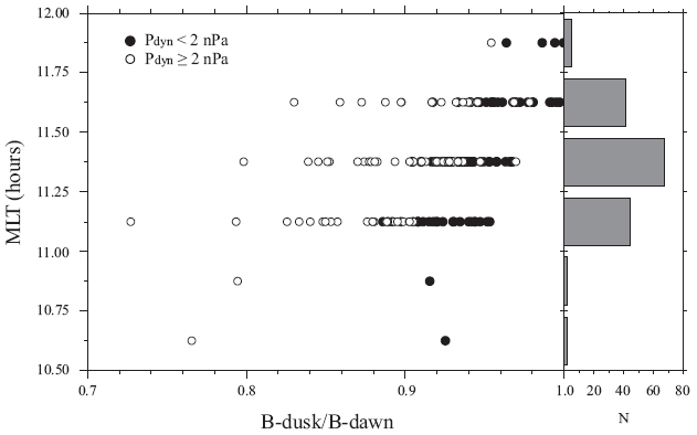
To statistically analyze how the peak location of the geosynchronous magnetic field is related with the changes of the solar wind dynamic pressure and the dawn-dusk asymmetry, the monthly geosynchronous magnetic field data were fitted to the second-order polynomial using the 15-min medians of the magnetic field data for the cases when the solar wind dynamic pressure was lower than 2 nPa, and at or higher than 2 nPa, and the peaks of the polynomial fitting curves were shown with respect to the dawn-dusk magnetic field median ratios of the corresponding months, as in Fig. 6. The number of distributed peak locations was shown in the histogram on the right. It was found in Fig. 6 that the peaks of the geosynchronous magnetic field data are usually located at 11:07, 11:22, and 11:37 MLT.

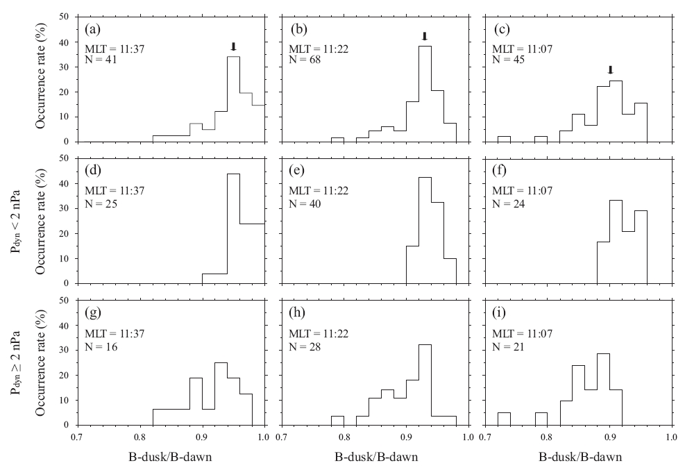
Using the data at these three MLTs, we statistically in-vestigated the correlation between the peak locations of the geosynchronous magnetic field data and the dawn-dusk asymmetry. Fig. 7 shows the distribution of the dawn-dusk magnetic field median ratios when the peaks of the geosynchronous magnetic field data were located at the time of (a) 11:37 MLT, (b) 11:22 MLT, and (c) 11:07

MLT. N denotes the total number of data points at corresponding MLT. We showed the percentage of the number of data points of the dawn-dusk magnetic field median ratio in each interval (0.02) to the total number of data points at each MLT. The Fig. 7a showed the maximum distribution at 0.95 of the dawn-dusk magnetic field median ratio, (b) at 0.93, and (c) at 0.90 (indicated by the arrows). This means that the peak location became farther away from the local noon as the dawn-dusk asymmetry was more significant.

To investigate how the observed peak location of the magnetic field is correlated with the solar wind dynamic pressure, analysis was performed for the cases where the solar wind dynamic pressure was lower than 2 nPa, and at or higher than 2 nPa. Figs. 7d-f show the distribution of the dawn-dusk magnetic field median ratios in the cases when the solar wind dynamic pressure was lower than 2 nPa, while Figs. 7g-i show that in the cases where the solar wind dynamic pressure was at or higher than 2 nPa. We found in Figs. 7d-f and g-i that the dawn-dusk asymmetry was more significant as the peak location became farther away from the local noon. In addition, it was verified between Figs. 7d and g, e and h, f and i that the dawn-dusk asymmetry was more significant in the cases when the solar wind dynamic pressure was great than in the cases when that was little. This indicates that the peak location of the magnetic field is dependent upon the changes of the solar wind dynamic pressure.

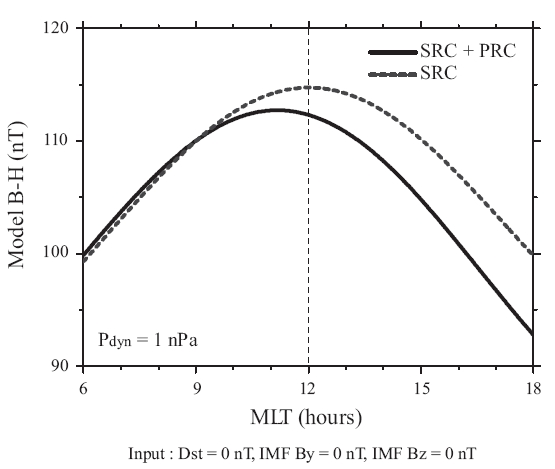
The TS-04 magnetic field model developed by Tsyganenko & Sitnov (2005) was employed to investigate the factors affect the morning-afternoon asymmetry of the magnetic field observed at the geosynchronous orbit and the peak location of the magnetic field in the geomagnetic field model. To investigate the effect of symmetric ring current (SRC) and partial ring current (PRC) in the geosynchronous orbit during the geomagnetically quiet time, TS-04 model values were calculated by putting in the solar wind dynamic pressure of 1 nPa, Dst of 0 nT, and the north-south component of the interplanetary magnetic field of 0 nT, as shown in Fig. 8. The line represents the H component magnetic field when the effect of both the SRC and PRC were taken into consideration, while the dotted line represents the H component magnetic field when only the effect of the SRC was taken into consideration. When only the SRC was taken into consideration, the peak of the magnetic field in the geosynchronous orbit was located near the local noon (12:00 MLT). How-

ever, when both the SRC and PRC were taken into consideration, the peak of the magnetic field was located in the morning sector (11:12 MLT). Additionally, the magnetic fields in the geosynchronous orbit were decreased in the afternoon sector. This indicates that the PRC that affects the geosynchronous orbit is mainly located at the outside of the geosynchronous orbit in the dusk sector. Hence, it is assumed that PRC may be the cause that moves the location of the peak in the geosynchronous orbit from the local noon toward the morning sector.

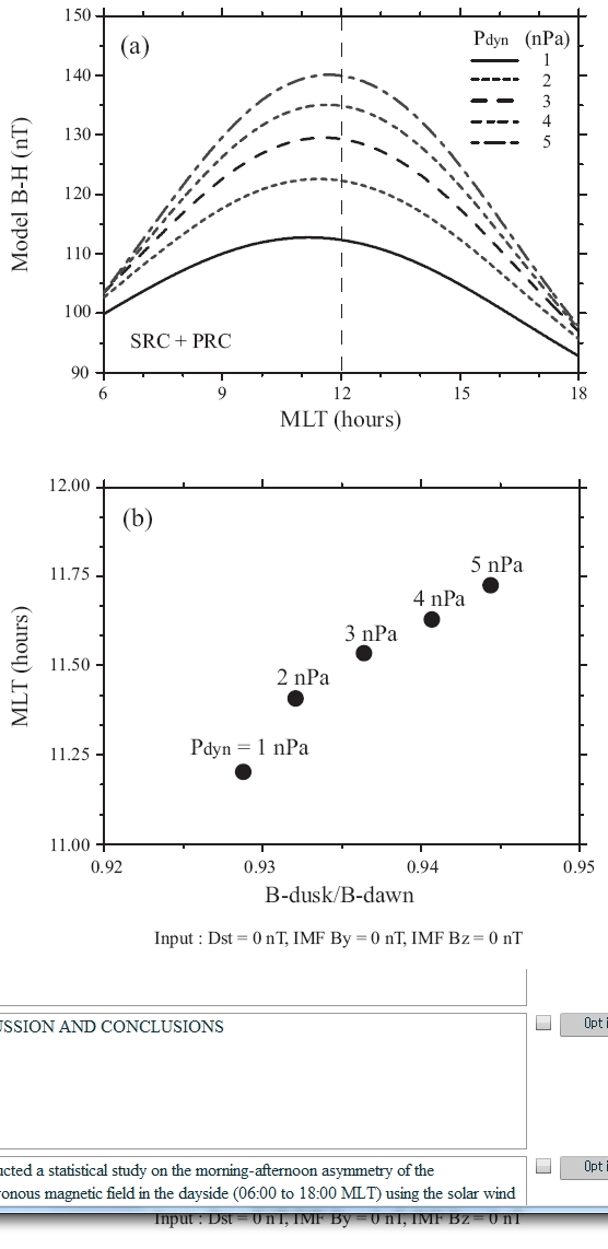
To investigate how the morning-afternoon asymmetry of the geosynchronous orbit by the PRC is changed by the changes of the solar wind dynamic pressure in the TS-04 model, the model values depending on the solar wind dynamic pressure were shown in Fig. 9a for each MLT. For the Dst and the north-south component of the interplanetary magnetic field, the same values used in Fig. 8 were employed. The solar wind dynamic pressure was

increased by 1 nPa from 1 nPa to 5 nPa. Different from the observation, it was found in the TS-04 model that the location of the geosynchronous magnetic field was moved toward the local noon region as the solar wind dynamic pressure was increased. To confirm this, the peak location of the TS-04 model values was shown in comparison with the dawn-dusk magnetic field median ratio as in Fig. 9b. It was verified that the dawn-dusk asymmetry became more significant as the peak of the magnetic field was moved farther away toward the morning sector. This tendency was consistent with the observation result shown in Fig. 7. However, in Figs. 9a and b, we found the tendency that the dawn-dusk asymmetry was decreased as the solar wind dynamic pressure increased, which was opposite result with the observation shown in Fig. 7. This may be because the effect of magnetopause current is dominant on the geosynchronous magnetic field in the day sector than that of the PRC when the solar wind dynamic pressure is increased in the TS-04 model.

We conducted a statistical study on the morning-afternoon asymmetry of the geosynchronous magnetic field in the dayside (06:00 to 18:00 MLT) using the solar wind data, the geosynchronous magnetic field data and the Kp index observed in the period between February 1998 and January 2007. Under the geomagnetically quiet time obtained from the Kp index, we observed the morning-afternoon asymmetry, which is that the peak of the geosynchronous magnetic field is located in the morning sector, not at the local noon (Fig. 2). To investigate whether or not the peak of the magnetic field was located in the morning sector by the effect of the solar wind speed and the Earth’s orbital motion speed, that is, the aberration effect, we compared the aberration angle and the peak location of the geosynchronous magnetic field calculated by using the Earth’s orbital motion speed and the solar wind speed data from the ACE satellite, and the result showed that the morning-afternoon asymmetry could not be accounted for only by the aberration effect (Fig. 4).

In the statistical analysis of the geosynchronous magnetic field, it was found that the peak location of the geosynchronous magnetic field was moved farther from the local noon toward the morning sector as the dawn-dusk asymmetry was more significant, in other words, as the dusk sector magnetic field (B-dusk) median was smaller than the dawn sector magnetic field (B-dawn) median (Fig. 7). In order to investigate the cause of the asymmetry, we employed the TS-04 model and examined the effect of the magnetospheric current. The effect of the ring current was investigated in the TS-04 model and the result showed that the afternoon sector magnetic field was smaller and the peak of the magnetic field was moved to the morning sector farther in the case when the effect of the PRC was taken into consideration than in the case it was not (Fig. 8). This indicates that the morning-afternoon asymmetry of the geosynchronous magnetic field is caused by the PRC that is more outstanding at the outside of the geosynchronous orbit in the dusk sector in the TS-04 model.

We also investigated how the relationship between the dawn-dusk magnetic field median ratio (B-dusk/B-dawn) and the peak location of the magnetic field is changed by the magnitude of the solar wind dynamic pressure. The relationship between the peak location of the geosynchronous magnetic field and the dawn-dusk magnetic field median ratio was compared and analyzed for the case when the solar wind dynamic pressure was lower than 2 nPa, and at or higher than 2 nPa, respectively (Figs. 7d-i). We found the tendency that the dawn-dusk magnetic field median ratio was lower in the case of large solar wind dynamic pressure (P_dyn ≥ 2 nPa) than in the case of little solar wind dynamic pressure (P_dyn < 2 nPa). This means the effect of the PRC is greater in the dusk sector when the solar wind dynamic pressure is great. However, we checked the geosynchronous magnetic fields depending on the variation of the solar wind dynamic pressure using the TS-04 model and the result showed that the dawn-dusk asymmetry was decreased as the solar wind dynamic pressure was increased (Fig. 9). This indicates that the effect of the PRC becomes relatively small as the effect of the magnetopause current in the dayside becomes more outstanding when the solar wind dynamic pressure is increased, which is not consistent with our observation result. Hence, the effect of the PRC should be considered more in the TS-04 model when the solar wind dynamic pressure is increased.

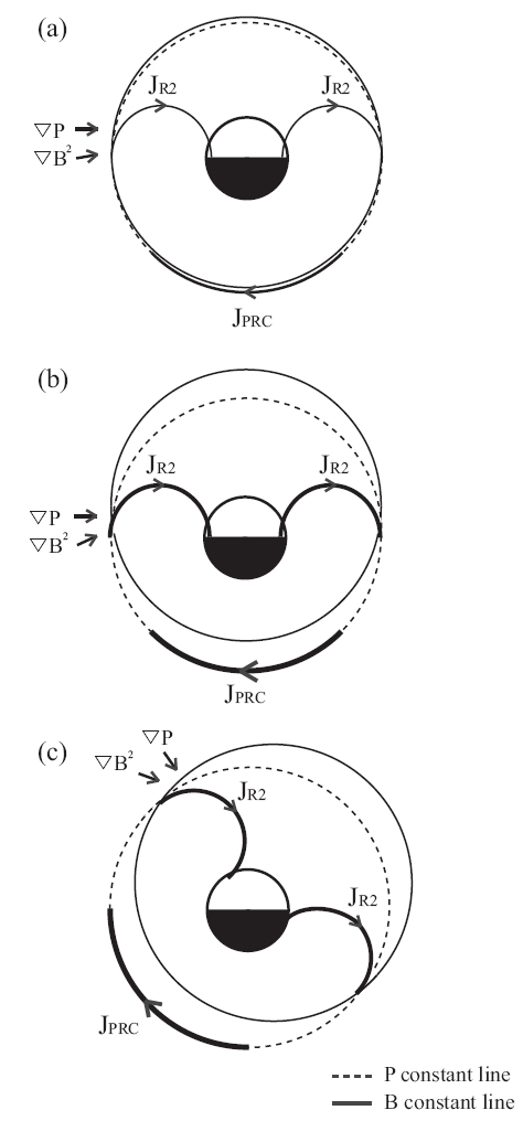
Since the PRC is closed by the Region 2 field-aligned current (Bakhmina & Kalegaev 2008), the region where the PRC is distributed is associated with the generation of the Region 2 field-aligned current (Nakano et al. 2009). Bostrom (1975) expressed the current density J_||,I of the Region 2 field-aligned current flowing to the ionosphere in the magnetohydrodynamic equilibrium state as Eq. (1):

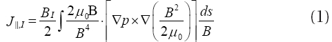
where B denotes the magnetic field vector, B the magnetic field strength, B_I the magnetic field strength at the point connected to the ionosphere, ρ the plasma pressure, μ₀ the permeability, and ds the infinitesimal length in the direction of the magnetic field. As in the equation above, the Region 2 field-aligned current is determined by the direction of the plasma pressure gradient and the direction of the magnetic pressure gradient, and generated in the form that connects the magnetosphere and the ionosphere. Nakano et al. (2009) mentioned that weak PRC is generated when the solar wind dynamic pressure is weak since the magnetosphere is weakly compressed and thus the directions of the plasma pressure gradient

and the magnetic pressure gradient are almost overlapped (Fig. 10a), while the magnitude of the PRC is increased as the solar wind dynamic pressure is increased since the magnetosphere is more compressed in the dayside and thus the directions of the plasma pressure gradient and the magnetic pressure gradient are different (Fig. 10b).

On the other hand, Lui (2003) observed the increase of the proton plasma pressure when the geomagnetic field is perturbed (Kp > 3₊) in the dusk to midnight sector (21:00 to 22:00 MLT). Lui also observed the distribution of the ratios of the magnetic field in the disturbed time to that in the very quiet time (B[Kp > 3₊]/B[Kp < 2]), and found that the PRC is asymmetrically distributed around the dusk-midnight sector when the geomagnetic field is perturbed. Using the Dst index in which the effect of only the ring current is considered, Le et al. (2004) observed the rotation of the center of the PRC maximum near the magnetic equator from the midnight sector to the dusk sector following the decrease of the Dst index. Cummings (1966), using the H-component (north-south) magnetic field data from a ground station located at a low latitude and determining the H-component magnetic field averages in the ground station for five quiet days in each month, observed that the cases when the difference between the averages and the H-component of each month in the ground station was more than 100 nT (H_{5-quite days}-H ≥ 100 nT) were found frequently in the dusk sector (18:00 MLT). Additionally, considering the fact that the H-component magnetic field in a ground station were decreased more in the dusk sector than in the dawn sector during the main phase of the magnetic storm by the effect of the PRC (Wolf et al. 2007), we suggest that there should be a close relationship among the rotation of the field-aligned current generation point by the change in the directions of the plasma pressure gradient and the magnetic pressure gradient, the change of the PRC generation point, and the morning-afternoon asymmetry of the geosynchronous magnetic field we observed.