Thermospheric neutral mass density, which primarily determines the atmospheric drag, is an important parameter for satellite operations in the near-Earth space, and is also very useful for understanding the thermosphereionosphere coupling process as well. The thermospheric neutral mass density is highly variable in space and time by various energy and momentum sources. In particular at high latitudes, these sources are directly or indirectly associated with the direction and/or strength of the interplanetary magnetic field (IMF) (McCormac & Smith 1984, McCormac et al. 1985, 1991, Killeen et al. 1985,1995, Meriwether & Shih 1987, Thayer et al. 1987, Rees &Fuller-Rowell 1989, 1990, Sica et al. 1989, Hernandez et al.1991, Niciejewski et al. 1992, 1994, Won 1994, Richmond et al. 2003, McHarg et al. 2005, Zhang et al. 2005, Kwak & Richmond 2007, Kwak et al. 2007, Luhr et al. 2007, Forster et al. 2008). Therefore, there is an intimate relationship between the IMF variation and thermospheric density variation (Crowley et al. 2006, Rentz & Luhr 2008, Kwak et al. 2009).

Recently, Kwak et al. (2009) have carried out the systematic analysis of observed IMF B_y and B_z influences on the thermospheric density by using the high-latitude southern summer thermospheric total mass density near 400 km altitude, derived from the high-accuracy accelerometer on board the Challenging Minisatellite Payload (CHAMP) spacecraft during October 17, 2001 through February 24, 2002. Their study showed that the thermospheric density distribution depends on the orientation of the IMF. Especially, their study showed that the difference in density distributions, which were obtained by subtracting values for zero IMF from these for non-zero IMF, varied strongly with respect to the direction of the IMF: density differences poleward of -50° tended to be strongest when B_z was negative, and stronger when B_y was negative than when it was positive. Density differences for negative B_y showed significant enhancements in the early morning hours and hours around dawn, but showed reduced values in the dusk sector. For positive B_y the density differences were opposite in sign to those for negative B_y. Density differences for negative B_z showed significant increases in the cusp region and premidnight sector, but a small decrease in the dawn sector. The density differences at high latitudes tended to be weakest when B_z is positive. Since the behavior of the high-latitude thermospheric densities varies with IMF conditions, one can expect that the sources driving the thermospheric density variations should vary with IMF conditions.

Further study is necessary to identify why the variation of the thermospheric neutral mass density is dependent on the orientation of the IMF. In this paper, we extend the work of Kwak et al. (2009) by conducting model simulations by using the coupled model of the National Center for Atmospheric Research Thermosphere-Ionosphere Electrodynamics General Circulation Model (NCAR-TIEGCM) and a new empirical model that provides a forcing of the thermosphere in high latitudes.

The TIEGCM (Richmond et al. 1992) used in this study is an extension of the NCAR-TIGCM (Roble et al. 1988) that incorporates the electrodynamic processes. The TIEGCM simulates self-consistently the neutral winds, conductivities, electric fields and currents. The model calculates the neutral gas temperature and mass mixing ratios of O₂, N₂, O, N(²D), N(⁴S), and NO. It also solves the electron and ion temperatures and the number densities of O⁺, O₂⁺, NO⁺, N₂⁺, and N⁺. The numeric grid size of the model is 5° × 5° horizontally and 1/2 scale height vertically, and the vertical coordinate has 29 constant pressure levels from approximately 97-700 km altitude. The external inputs required by the model are the solar extreme ultraviolet (EUV) and UV fluxes, the auroral particle precipitation, the ionospheric convection, and the upward propagating tides from the middle atmosphere.

The model simulations are conducted by using the seasonal and solar conditions on January 5, 2002. The F10.7 index was 224 × 10^-22 W/m²/Hz and the total hemispheric power (HP) was 16 GW on that day. The HP is related with Kp index by HP (GW) = -2.78 + 9.33 × Kp (Maeda et al. 1989). The mean Kp index on January 5, 2002 was 2. The prescriptions of the upward propagating diurnal and semidiurnal tides are taken from the Global Scale Wave Model (GSWM) (Hagan & Forbes 2002). The TIEGCM used in this study is coupled with a new empirical model of the high-latitude forcing on the thermosphere including electric field, magnetic potential and Poynting flux, and soft particle precipitation to the polar region (Deng et al. 2008) is considered.

To investigate the response of the thermospheric density to varying IMF, we made five TIEGCM simulations for IMF (B_y, B_z) values of (-4.4, 0.0), (4.4, 0.0), (0.0, -3.4), (0.0, 3.4), and (0.0, 0.0) nT. The magnitudes of the non-zero reference values of B_y and B_z (4.4 nT and 3.4 nT). The 4.4 and 3.4 nT are the root-mean square values of B_y and B_z corresponding to the IMF on the day that Kwak et al. (2009) analyzed the CHAMP neutral mass density data. We have chosen those IMF values to compare the model simulation results with the CHAMP data. A 2-min time step is used for the entire simulation, and linear interpolations of input values are made at a given time step. The TIEGCM history is recorded hourly for January 5, 2002.

Quantities considered to investigate the potential source of the variation of the neutral mass density in the high latitudes are E × B drifts, neutral winds, and heating terms including auroral heating and joule heating. We first bin each quantity at 400 km altitude for each universal time in magnetic coordinates for different orientations of the IMF; we analyze the quantities in Quasi-Dipole (QD) coordinates (QD-latitude and magnetic local time [MLT]) (Richmond 1995). Especially, for analysis of E × B drifts and neutral winds, the QD-latitude/MLT region poleward of 47.5°S is divided into 145 subregions of approximately equal size, each having 5° width in latitude, and a variable, latitude-dependent, width in MLT. The number of MLT subregions at a given latitude decreases from 32 at 50°S to 4 at 85°S, plus one at the pole.

We then carry out an averaging for 24 UT hours of each quantity in each bin for each of the different IMF conditions. The resultant values can be then mapped out over magnetic latitude and MLT.

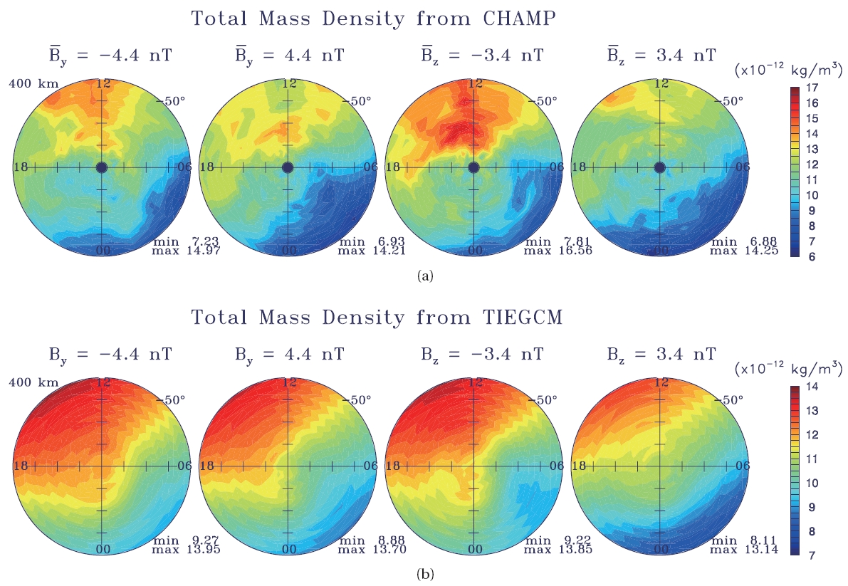
To examine how well the thermospheric densities from the TIEGCM agree with the observations, we compare the results of the TIEGCM with densities derived from

the high-accuracy accelerometer on board the CHAMP spacecraft as analyzed by Kwak et al. (2009).

Figs. 1a and b show the average thermospheric neutral mass densities at 400 km over the southern summer hemisphere in the poleward latitude -50° for IMF (B_y, B_z) values of (-4.4, 0.0), (4.4, 0.0), (0.0, -3.4) and (0.0, 3.4) nT from CHAMP observations and the TIEGCM run, respectively. These projections are as if one were looking up on the thermosphere from below. For all IMF conditions, southern summer high-latitude thermospheric total mass density at 400 km from the CHAMP shows the classic picture, reaching a maximum in the postnoon sector (~14 MLT), and a minimum in the early morning sector (~04 MLT). Density patterns having the postnoon maximum and early morning minimum at high latitudes have been seen in previous studies (Jacchia & Slowley 1968, Liu et al. 2005). And large thermospheric density peaks is clearly visible in the cusp region. This feature is most pronounced when the IMF B_z is negative. This feature and its strengthening with increasing magnetic activity were also reported in previous studies (Luhr et al. 2004, Liu et al. 2005, Rentz & Luhr 2008). The TIEGCM thermospheric density distributions show agreements with the CHAMP observations for the dependence of density on the IMF direction, although variations in the model density are generally weaker than observations and don’t show the significant large peak in the cusp region as do the observations. This difference may be associated with numerical smoothing features of the model.

The general agreement between thermospheric density observations and model results indicates that we can use the model to analyze in more detail the sources that drive the neutral density variations in the summertime high-latitude thermosphere.

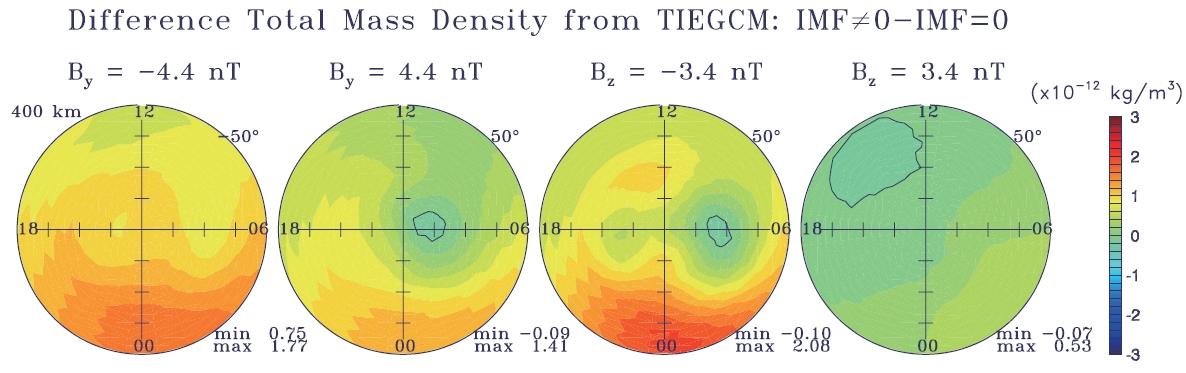
Fig. 2 shows the difference of thermospheric neutral mass densities (subtraction of the values for zero IMF condition from the values for non-zero IMF conditions) at 400 km over southern-hemisphere high latitudes for the four IMF (B_y, B_z) values from the TIEGCM run. As shown in Fig. 2, the thermospheric density variation patterns in the high latitudes depend on the orientation of the IMF. The difference densities for negative B_y show an increase in almost the whole polar regions. In particular, there are significantly enhanced densities in the dusk sector and around midnight when B_y is negative. Under the positive-B_y condition, although there is an increase of difference density in the afternoon including midnight, there is a decrease in the early morning hours including the dawn side poleward of -70°. The difference of the thermospheric densities for negative B_z shows a strong enhancement in the cusp region and around midnight with maximum value of 2.08 × 10^-12 kg/m³, but decreases in the dawn sector. In the dusk sector, although densities are not significantly enhanced, those

values are relatively larger than those in the dawn sector. The positive-B_z difference densities show decreases generally, although there are weak increases in the early morning and evening sectors. The negative-B_z difference densities are more significant than the positive-B_z difference densities, indicating that negative B_z has a stronger effect on the thermospheric density than does positive B_z. Since the behavior of the high-latitude thermospheric densities varies with IMF conditions, one can expect that the sources driving the thermospheric density variations should vary with IMF conditions.

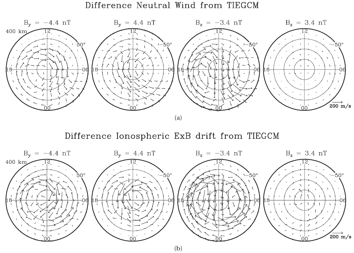
A possible interpretation for different thermospheric density patterns for different IMF conditions is that the high-latitude thermospheric density is strongly determined by thermospheric winds, which are associated with the ionospheric convection and vary strongly with respect to the direction of the IMF. Geostrophic adjust theory, as it applies to the thermosphere (Larsen & Mikkelsen 1983, Walterscheid & Boucher 1984), indicates that winds and horizontal pressure gradients tend to be linked, such that a cyclonic wind vortex tends to have a low pressure and density at its center, while an anti-cyclonic vortex tends to have a high pressure and density at its center.

Fig. 3 shows the difference of neutral winds and difference ionospheric convection velocities at 400 km over southern hemisphere high latitudes for four IMF (B_y, B_z) values. The difference winds reflect well the pattern of the difference ionospheric E × B drifts with different IMF conditions, indicating that the thermsopheric winds are influenced strongly by ionospheric plasma convection

through the ion drag. The difference winds for negative B _y show a strong high-latitude anticyclonic vortex on the dusk side. The difference winds for positive B_y show a high-latitude cyclonic vortex on the dawn side. The difference neutral winds for negative B_z have a two-cell structure with evening anticyclonic and morning cyclonic vortices, and extend to subauroral latitudes. There is an equatorward flow in the early morning hours. The negative-B_z difference winds are stronger than the positive-B_z difference winds, indicating that negative B_z has a stronger effect on the winds than does positive B_z.

If the geostrophic adjust theory is applied to the thermosphere, we would expect strong anticyclonic winds on the dusk side for negative-B_y condition drive high neutral density on the dusk side of the polar cap. We also expect that strong cyclonic winds on the dawn side drive low neutral density on the dawn side for positive-B_y condition. This speculation generally agrees with the density distributions in Fig. 2. Similarly, the dawn-side minimum difference density around -70° for negative B_z, and maximum difference density for positive B_z, are related to the strength of the cyclonic vortex there seen in Fig. 3. In contrast, the difference densities around 18 MLT are not much larger for negative B_z than for positive B_z, despite the fact that the dusk-sector anti-cyclonic winds having high pressure and density shown in Fig. 3 are considerably stronger for negative B_z than for positive B_z. The possible reason can be that the horizontal advection of momentum, or centrifugal force, is strongly divergent in the dusk sector for B_z negative, reducing the need for an outward pressure-gradient force to help balance the Coriolis force, and decreases density in the dusk sector (Kwak et al. 2007). Eventually, high-latitude thermospheric density, especially in the dawn and dusk sectors, can be strongly determined by thermospheric winds, which are associated with the ionospheric convection and vary strongly with respect to the direction of the IMF.

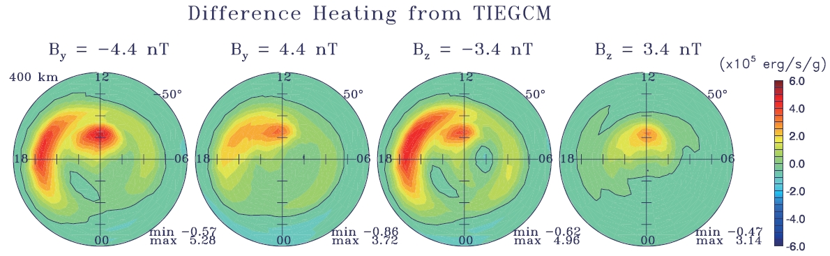
Additionally, thermospheric density variations can be also influenced by the local heating including joule heating and auroral heating associated with ionospheric currents and/or auroral particle precipitation, which vary with IMF conditions. Indeed, the heating may generate upward neutral motion and cause an increase of total mass density.

Fig. 4 shows difference heating terms at 400 km altitude over the southern hemisphere for IMF (B_y, B_z) values. For negative B_y, a strong difference heating occurs in the auroral region in the afternoon and polar cusp region with the maximum value of 5.28 × 10⁵ erg/s/g. For positive IMF B_y, the distribution of the difference heating is similar to that for negative B_y condition but the intensity with maximum value of 3.72 × 10⁵ erg/s/g is weaker than that for negative B_y. For negative IMF B_z condition, there is also a strong difference heating regions in the afternoon and polar cusp region with the maximum value of 4.96 × 10⁵ erg/s/g. When positive IMF B_z condition, a weaker difference heating than that other IMF conditions occurs around polar cusp region with the maximum value of 3.14 × 10⁵ erg/s/g.

If these difference heating distributions are considered with the thermsopheric density distributions from Fig. 2, we can see the high-latitude thermospheric density variations in auroral and cusp regions, especially near cusp region for negative B_z condition, are also influenced by the local heating associated with ionospheric currents and/or auroral particle precipitation, which vary with IMF conditions. Luhr et al. (2004) suggested Joule heating due to very intense small-scale field aligned currents (FACs) near the cusp region at a lower level causes upwelling and enhanced neutral mass densities at a higher level. In particular, Neubert & Christiansen (2003) pointed out that small-scale FACs are strong in the cusp region when the IMF is strongly southward, which may explain why strong thermospheric density distributions near the cusp region occur for negative B_z. Recently, it has been shown by Rentz & Luhr (2008) that the increased positive anomaly in cusp density is detected for about an hour after the enhancement of the merging electric fields, which are proportional to amplitude of southward IMF.

In this paper, we present the investigations of the driving sources for the high-latitude thermospheric density variations depending on the IMF conditions. For this study, we analyzed steady state condition for different IMF directions, for summer conditions in the southern hemisphere, on the basis of numerical experiments with the NCAR-TIEGCM coupled with a new quantitative empirical model of the high-latitude forcing on the thermosphere.

The difference high-latitude thermospheric densities, obtained by subtracting values with zero IMF from those with non-zero IMF, vary with IMF conditions: There are significantly enhanced difference densities in the dusk sector and around midnight when B_y is negative. Under the positive-B_y condition, there is a decrease in the early morning hours including the dawn side poleward of -70°. For negative B_z, the difference of the thermospheric densities shows a strong enhancement in the cusp region and around midnight, but decreases in the dawn sector. In the dusk sector, those values are relatively larger than those in the dawn sector. The density difference under positive-B_z condition shows decreases generally. The density difference is more significant under negative-B_z condition than under positive-B_z condition.

A possible interpretation for different thermospheric density patterns for different IMF conditions is that the high-latitude thermospheric density, especially in the dawn and dusk sectors, can be strongly determined by thermospheric winds, which are associated with the ionospheric convection and vary strongly with respect to the direction of the IMF: Strong anticyclonic winds on the dusk side for B_y negative condition drive high neutral density on the dusk side of the polar cap. For positive B_y, strong cyclonic winds on the dawn side drive low neutral density on the dawn side. The dawn-side minimum difference density for negative B_z, and maximum difference density for positive B_z, are related to the strength of the cyclonic vortex. The difference densities around 18 MLT are not much larger for negative B_z than for positive B_z, despite the fact that the dusk-sector anti-cyclonic winds are considerably stronger for negative B_z than for positive B_z. Additionally, the high-latitude thermospheric density variations, especially in auroral and cusp regions, are also influenced by the local heating associated with ionospheric currents and/or auroral particle precipitation, which vary with IMF conditions.