Imaging spectroscopy or integral field spectroscopy provides spectral information at every angular position in a field. The resulting product is a three-dimensional(3D) data cube which comprises spatial information of the observed object in two dimensions and spectral information in the other dimension. The history of imaging spectroscopy in the near-infrared (NIR) is relatively short,but its potential of applying to various astrophysical issues had already been proven (see Weitzel et al. 1996 and references therein). For example, this observing technic is powerful to build emission line maps of extended objects since both the spectral lines and continuum are observed together at the same time, in the same spectroscopic format, and at each position, and the continuum is effectively subtracted using adjacent pixels along the spectral axis of the data cube. It is superior to the imaging technic using narrow-band filters particularly in such a crowded region as the Galactic center or massive starforming regions where seeing variation prohibits accurate continuum subtraction (Burton & Allen 1992, Lee et al. 2005).

To meet increasing demand in the community, a number of integral field NIR spectrographs with integral field units or image slicer units have been developed and currently in operation; including Gemini/NIFS (McGregor et al. 2003), VLT/SINFONI (Eisenhauer et al. 2003), and Keck/OSIRIS (Larkin et al. 2006). Slit scanning (stepping the slit position of a normal spectrograph across the target)is another method for imaging spectroscopy. Even though this technique is affected by seeing variations, we can observe large extended objects with long-slits or take very high spectral resolution spectra. We plan to apply this observing technique to cross-dispersed high resolution IR spectrographs such as Immersion GRating INfrared Spectrograph (IGRINS; Yuk et al. 2010) and Giant Magellan Telescope Near-Infrared Spectrograph (GMTNIRS;Lee et al. 2010).

The advantages of high dispersion spectrographs in the integral field modes enable us to study kinematics. For example, Lee et al. (2008) surveyed the circumference of Sgr A East in the Galactic center using the slit scanning technic in H₂ 1-0 S(1) (λ = 2.1218 ㎛m) line emission at a high resolving power (λ / λΔ ？ 18000). This remnant of an energetic explosion is colliding with the ambient material, and line profiles observed toward the shocked gas show its high velocity expanding motion (Lee et al. 2003). Thus Lee et al. (2008) chose high dispersion echelle for the spectroscopic configuration in their observations. The resulting data cube contains information of both structure and kinematics of the shocked H₂ gas with high-resolution line profiles at every spatial position. The data in the cube are continuous in the spatial dimensions as well as in the spectral dimension, i.e., along the velocity axis.

A conventional method of reducing the integral field observations is simply stacking two-dimensional (2D) spectral images into a data cube. For example, Burton & Allen (1992) and Lee et al. (2005) made use of only small portion of their data cubes along the spectral dimension; several slice images in some emission lines. In Lee et al. (2008), however, a unified data cube is required to investigate the entire survey region as a single system, since position and orientation of the slit in their observations changes along the circular boundary of Sgr A East. This type of slit-scanning observation at a high spectral resolution with a complicated survey scheme requires a new technic for data reduction.

In this paper, we introduce the sample data acquired by Lee et al. (2008) in Section 2, and describe in detail the process of data reduction for IR spectroscopy in Section 3. Section 4 presents a new technic for constructing a data cube.

Lee et al. (2008) surveyed the boundary region of Sgr A East in the H₂ 1-0 S(1) emission line which is radiated from shocked gas in the surrounding molecular clouds. They used the Cooled Grating Spectrometer 4 (CGS4; Mountain et al. 1990) at the 3.8 m United Kingdom Infrared Telescope (UKIRT) to observe the H₂ line profiles with an echelle grating and a 0.83 arcsec slit width. By the advantage of the long (~90 arcsec) slit length of CGS4, Lee et al. (2008) were able to scan the large area around Sgr A East with such a high spectral resolution.

Slit scanning observations were implemented in 3 arcsec steps. At the same time, the telescope was nodded between object and blank sky positions every 20 minutes to subtract background and telluric OH line emission. Fifty-six slit positions in total were observed over 11 fields around Sgr A East. The slit position angle was various from -90° to +40° (from north to east). HR 6496 and BS 6310 were observed as standard stars, which are used for flux calibration and distortion correction. More details on the observations can be found in Lee et al. (2008).

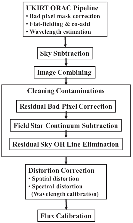
Basic data reduction steps, including bad-pixel-mask correction and flat-fielding (using an internal blackbody lamp), were accomplished by the automated Observatory Reduction and Acquisition Control (ORAC) pipeline at UKIRT. IRAF was used for the remaining part of the reduction process for 2D (wavelength and position) spectral images at individual slit positions. Stacking and making mosaic of those 2D spectral images into a 3D data cube and the later parts of reduction and analysis thereafter are implemented using Multichannel Image Reconstruction, Image Analysis and Display (MIRIAD; Sault et al. 1995, Hoffman et al. 1996). Flux calibration is

not included in this paper but described in detail in Lee & Pak (2006).

Sequence of data reduction of 2D spectral images using IRAF is shown in Fig. 1. Some steps in the sequence will be described in more detail in the following subsections. This reduction sequence can be modified alternatively depending on observing techniques. For example, if target position was jittered, distortion correction should be done before un-jittering (aligning) the images to be combined. Otherwise the distortions would spread out and become uncorrectable.

The wavelength range of 12.5 ㎛ is crowded with a dense forest of telluric OH lines. These emission lines come from a thin layer of the atmosphere at an altitude of about 90 km, and the strength of emission can vary rapidly; by a factor of two or more in half an hour duration (McLean 1997). There are also very strong OH lines near to our objective H₂ lines; stronger by orders of magnitude and as close as a few hundred km s^-1 apart. Sky OH lines are not subtracted perfectly because of their nature of rapid variations. The high spectral resolving power of CGS4 enables the target H₂ emission line to be separated from the brightest residual OH lines. However, in our case, we found that velocity dispersions of the observed H₂ lines are so large that wings of the H₂ 10 S(1) lines in some spectral images are slightly overlapped with the nearest OH line (at λ = 2.1232424 ㎛ which is ~200 km s^-1 apart from the H₂ line; Rousselot et al. 2000).

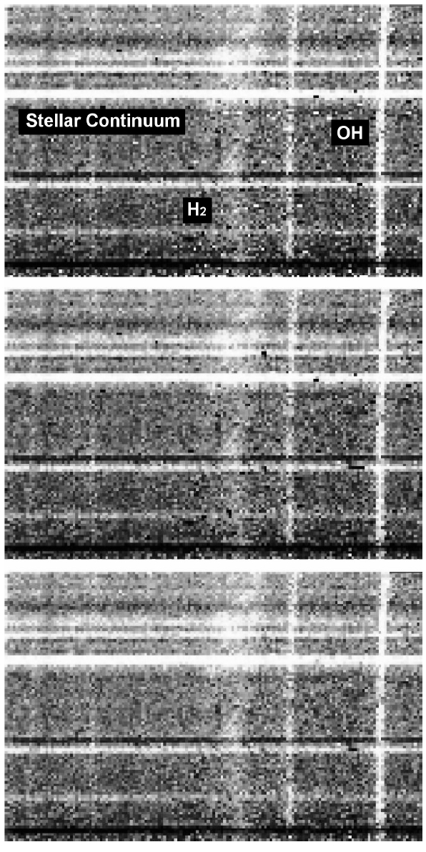
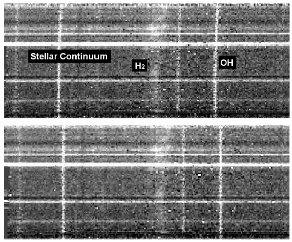
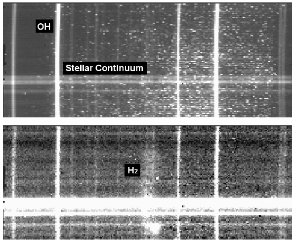
By subtracting a blank sky image from an object image, the background signals including telluric OH lines are diminished. Fig. 2 shows the image before (top figure) and after (bottom figure) the subtractions. Vertical lines are telluric OH lines and horizontal lines are stellar continua. After subtracting the blank sky image, diffuse H₂ emission becomes visible in the central part of the image. Since the background and strong OH lines are diminished, stellar continua look more prominent. Dark horizontal lines in upper part of the bottom figure are the scars due to the stellar continua in the sky image. Note also that the number of serious bad pixels is obviously decreased but many of them still remain and a lot of over-subtracted pixels newly appear as black points. They are typically stronger than diffuse H₂ emission and still contribute as serious contaminations.

On the other hand, since the Galactic center is an extremely crowded region, not surprisingly a number of stellar continua are included in each spectral image. Typ-

Typically two or three of them are much brighter than the H2 emission (Fig. 2). Therefore those contaminations should be cleaned up to obtain pure H2 spectra with high signal-to-noise (S/N) ratios.

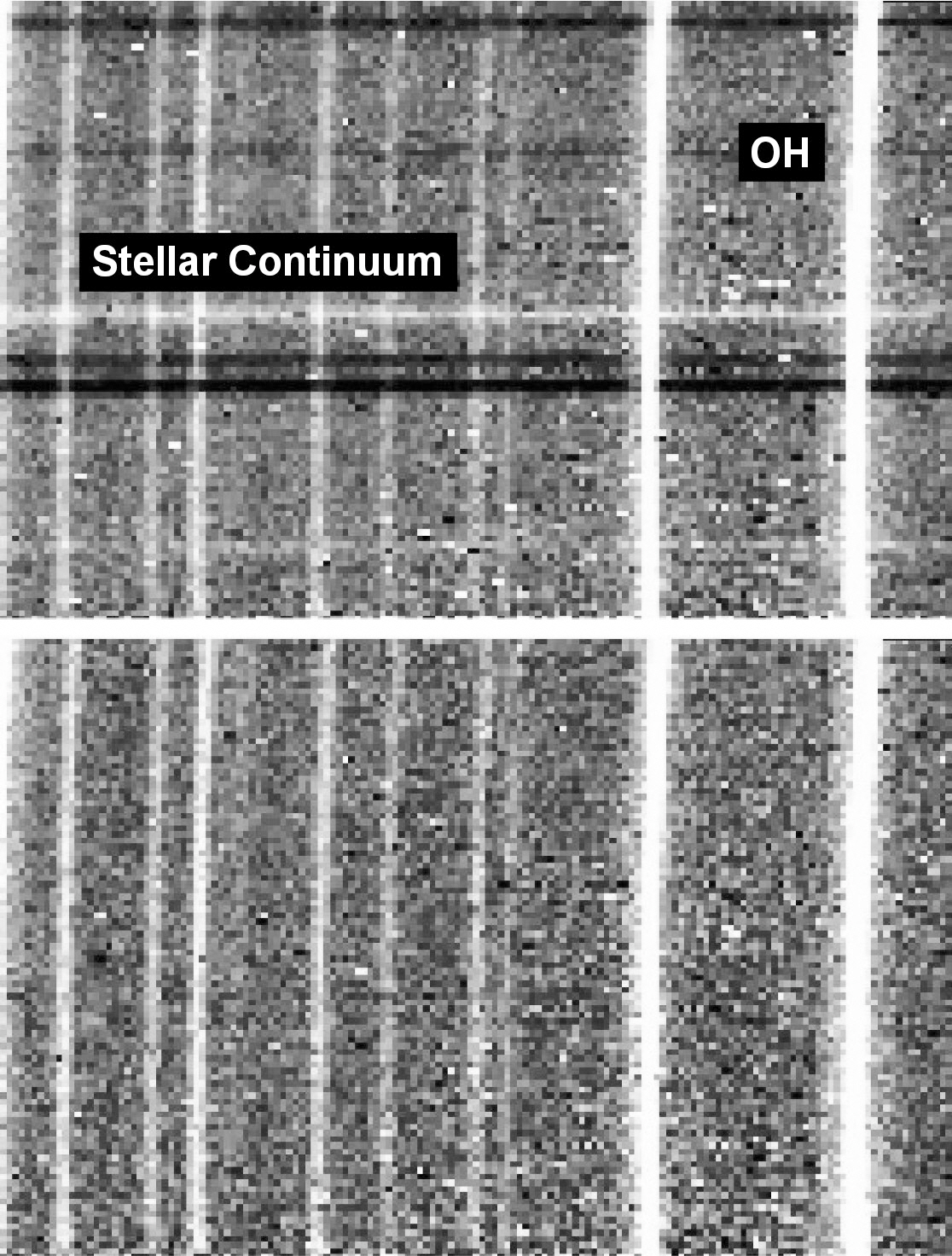
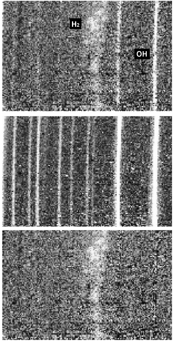
The residual bad pixels are corrected by using the IRAF package, NOAO.IMRED.CCDRED. COSMICRAYS, which detects cosmic rays or bad pixels in an image and replaces them with the average of neighboring pixels. We implement this task two times for each image. In the first run, bad pixels with positive values are corrected. Then, to take care of bad pixels with negative values, which are by-products of sky subtraction, we invert (multiply by -1) the once-corrected image and run COSMICRAYS again. By inverting the resulting image again to its original sign, the cleaning process for bad pixel completes (Fig. 3).

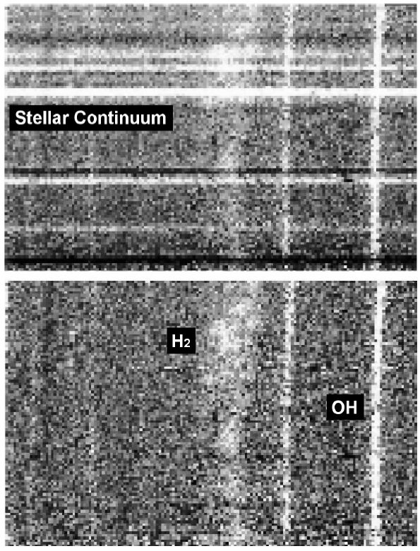
To remove continuum spectra of field stars, we use the IRAF package, NOAO.IMRED. GENERIC.BACKGROUND. Along each pixel row or column in an image, this task fits the background to a functional form and subtracts it. We apply linear fitting functions on both sides (at shorter and longer wavelengths) of the H₂ emission line in each row in each image. As a result, stellar continua are subtracted successfully around the emission line (Fig. 4).

In order to clean up the residual telluric OH lines, we need a template image of OH lines which will be scaled to have identical intensity levels with the residual OH lines and then be subtracted from the object image. A blank sky image can be used as a template. However, it includes the dark and sky background which was already subtracted from the object image by the process of sky sub-

traction above. Thus, we make a template image of pure OH lines by subtracting a mode value of the background from the blank sky image. This template image, however, still contains contaminations. Therefore we clean up the template image (Fig. 5) before we use it to remove the residual OH lines in the object image (Fig. 6).

The sequence in the cleaning process (bad pixel - stellar continuum - telluric OH lines) is determined irreversibly. The correction for bad pixels should be done before removing OH lines, otherwise the bad pixels in the OH template will be added to the object image and we will

lose or spoil a number of meaningful pixels. Also the stellar continuum subtraction should be done before OH correction to scale the template accurately to the object image. We found that it is better to correct bad pixels before subtracting continuum. It probably makes the continuum fit better. The cleaning process should be done before correcting spatial and spectral distortions since the distortion correction ;distort' original features in the images. Particularly it makes bad pixels larger and much more difficult to be identified and removed by COSMICRAYS.

To analyze the long slit spectrum, we should correct spectral distortion along the dispersion axis (i.e. curved stellar continuum) and spatial distortion along the slit (i.e. tilted or curved arc or telluric OH lines). In this stage of data reduction, IRAF tasks IDENTIFY, REIDENTIFY, FITCOORDS, and TRANSFORM in the package of NOAO.TWODSPEC.LONGSLIT are utilized. The correction for spectral distortion accompanies wavelength calibration as well.

For the correction of spectral distortion, we use spectrum of the standard star as a template. In principle, to fix distortions in the spectral direction, a standard star needs to be observed at different positions along the slit. However, since the spectral distortion of CGS4 in its echelle mode is not so serious (actually nearly negligible around the interested H₂ line), stellar spectra obtained at two or three positions are enough to make a template. Typically, stars are jittered along the slit to subtract the sky background (by subtracting the jittered image from the original image). With one jittering, we get two templates (e.g. template 1 and template 2), each of which contains one stellar spectrum at the different position, respectively.

The procedure of spectral distortion correction is as follows. First, we use IDENTIFY to mark the position of the standard star spectrum across the central column in template 1. Second, we measure the position of the same standard spectrum across different columns in template 1 using REIDENTIFY. Then we repeat IDENTIFY and REIDENTIFY on template 2. Using the task FITCOORDS, we find a transformation solution for the distortion in the dispersion direction evident in these standard spectra. Finally, after verifying the solution using the standard star images first, we transform the object images using TRANSFORM.

In a very similar way we correct for distortions in the spatial direction. First, we run IDENTIFY on the sky OH spectra (across the central row this time) and input the wavelength of each OH line. We use four OH lines (at 2.1156116 ㎛, 2.1176557 ㎛, 2.1232424 ㎛, and 2.1249592 ㎛) for the H₂ 1-0 S(1) spectral images. These telluric OH lines are bright enough for their pixel positions along the dispersion axis to be measured with a high accuracy and their wavelengths can be found in the literature (Rousselot et al. 2000). Next, we run REIDENTIFY, FITCOORDS, and TRANSFORM just like in the correction for spectral distortions. In Fig. 7, we show an example of the distortion correction.

We also calibrate wavelength of the data during the correction of spatial distortions, using known OH lines

as references. The information of calibrated wavelength is written in FITS headers as coordinate along the axis of spectral dispersion. Then we can convert wavelength into velocity relative to the rest wavelength of H₂ line using NOAO.ONEDSPEC.DISPTRANS. We can also correct for the motions of the Earth and Sun using ASTUTIL.RVCORRECT in order to determine local standard of rest (LSR) velocities.

The reliability of the wavelength calibration was verified by estimating its accuracy and precision. For accuracy, we measure calibrated wavelengths of all available OH lines in the sky images and compare them with known values (Rousselot et al. 2000). Then the average of the resulting differences is about ±0.5 km s^-1. For precision, we calculate dispersion of measured wavelengths for the OH line at 2.1232424 ㎛ which is nearest to the H₂ 1-0 S(1) line (2.1218 ㎛). Then the resulting dispersion is as large as ±1 km s^-1.

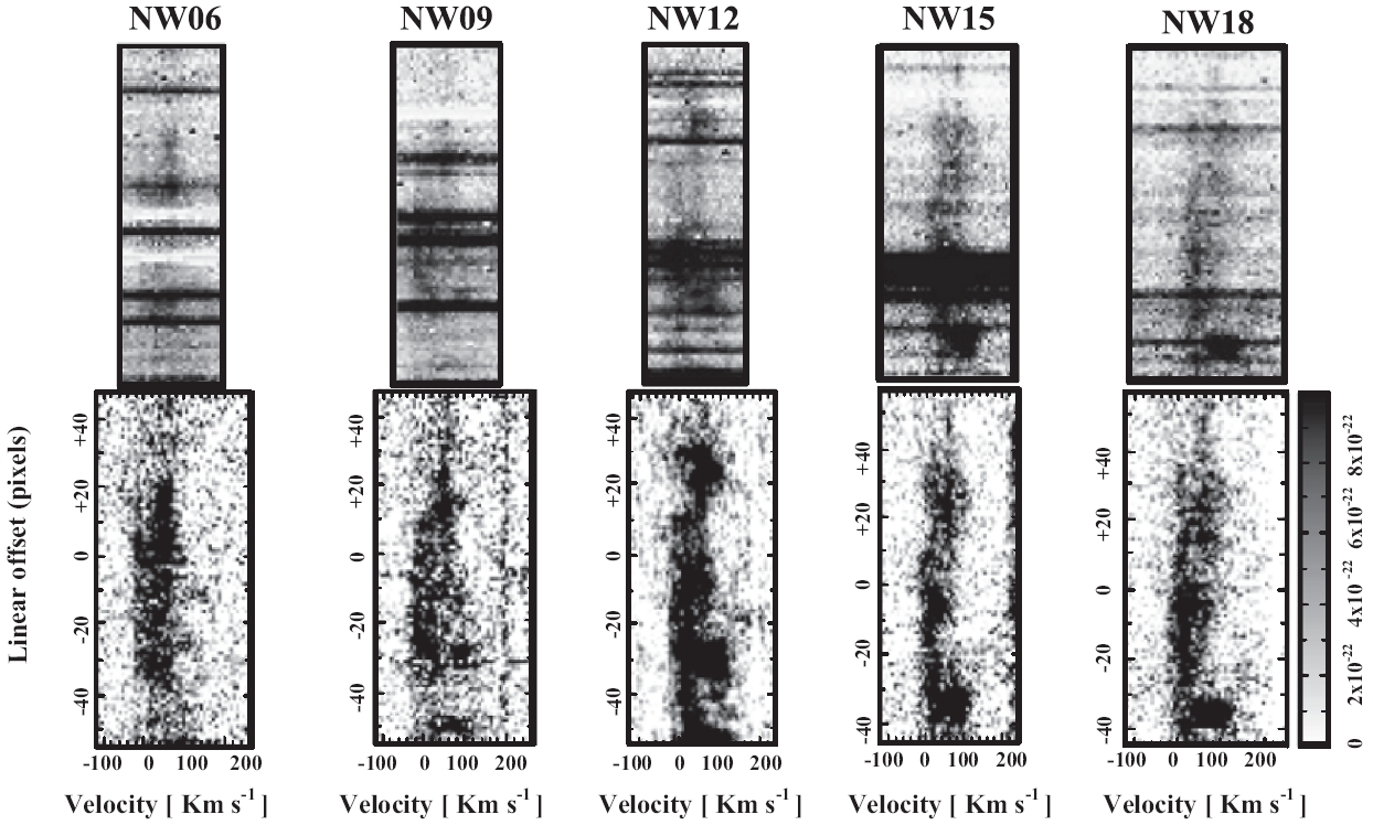
Selected from the 2-D spectral images we observed in the northern part of Sgr A East, several raw (only sky-subtracted) images and their reduced results are compared with each other in Fig. 8.

By unifying the high resolution 2D spectral images into a 3D data cube, we can investigate the structure and kinematics of the H₂ emitting gas simultaneously. At the wavelengths shorter than IR, 3D observations with such high spectral resolutions using echelle grating as in our case have not been so popular. However, in radio observations, it is not unusual to map a large area with a very high resolution in frequency. Thus there are some useful tools for reducing and handling 3D data.

MIRIAD (Sault et al. 1995, Hoffman et al. 1996) is a radio interferometry data reduction package, in the user environment with a large set of moderate-sized programs which perform individual tasks, involving calibration, mapping, deconvolution and image analysis of interferometric data. However, MIRIAD can also be used for general reduction of continuum and spectral line data in various formats (including FITS) throughout all stages of image analysis and output. Hence we choose MIRIAD for our near-IR 3D data reduction.

First, we have to transform the FITS data reduced by IRAF into the MIRIAD data format. This transformation of data format is easily achieved by the MIRIAD task FITS. This task also translates some standard information contained in the header of the FITS files into a MIRIAD-readable format (called ‘item’). However, the FITS task cannot understand all the ;fields' in the original FITS header since the definitions are often different between

observatories or instruments. Thus we need to manually translate some necessary FITS fields into MIRIAD items.

Then we use the MIRIAD task IMCAT to stack the 2D spectral images into a single 3D data unit (or data cube). We build data cubes separately for individual slit-scanning group since spectral images in each group are all the same in dimension and share a common position reference and slit angle. As a result, 11 data cubes with different dimensions, positions, and inclination angles are built from the entire survey area.

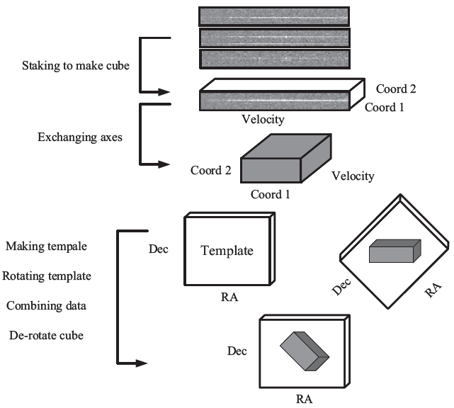
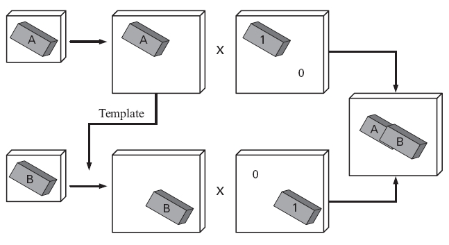
However, in order to investigate the large-scale structure in the surveyed region, we need to combine the unit data cubes into a single and global data cube. For this purpose, every pixel in each unit data cube should know its exact position on the sky; i.e. we need to set coordinate information on each data cube. The sequence of this process is presented in Fig. 9. As seen in the figure, the simply stacked data cubes have two spatial axes; one along the slit length and the other along the slit-scanning direction. If the slit position angle is simply a multiple of right angle (i.e. 0°, 90°, 180°, and 270°), those two axes could be directly projected on Right Ascension (R.A.) and Declination (Dec), respectively, or vice versa. However, in our observations with various slit position angles, this coordinating process becomes slightly complicated. First, we make a template cube which contains no data value but is defined in celestial coordinates (R.A. and Dec) along two spatial axes. Second, we rotate the template by the slit position angle. Third, we merge the data cube with this rotated template cube. Finally, we de-rotate the merged cube so that each data pixel is located at its exact position on the sky.

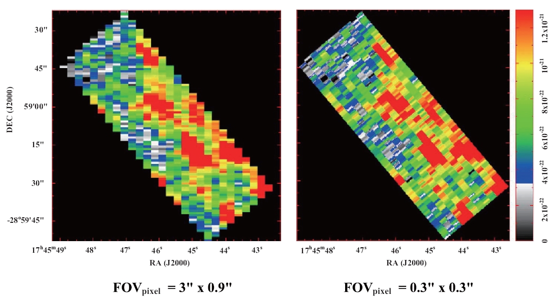
Before the coordinating process above, we should re-sample the data cube along all its three axes using the MIRIAD task REGRID. The original pixel scale in the data cube, which is determined by the mapping resolution of the slit scanning, is not in a square shape but 0.9" × 3" along the slit length and perpendicular to it, respectively. Thus the intensity distribution could become biased after rotation of the cube. To minimize this bias effect, we divide each pixel into much smaller, square, pixels with a scale of 0.3" × 0.3" (Fig. 10). This higher sampling resolution has another merit of more accurate matching when we combine the individual data cubes into the global cube. For this unification, we also re-sample and unify the velocity axes of the data cubes into a common definition (68 pixels with a scale of 7.3 km s^-1 in the range from -200 to +300 km s^-1).

MIRIAD has several tasks for mosaicking data cubes. Among them LINMOS is the most appropriate task for

non-radio type data like ours. However, while using LINMOS for mosaicking data cubes, we found problems in overlapped regions (Fig. 11). Since the pixel values in the overlapped region are averaged by LINMOS, when an observed position in one cube is overlapped by a blank position in another cube, the averaged pixel value in the combined cube becomes only a half of what should be. The blank regions are byproducts from the cube rotation, but MIRIAD regards the pixel values in those blanks as meaningful zero.

Thus we implement a ‘weighted mosaic’ for our data cubes;

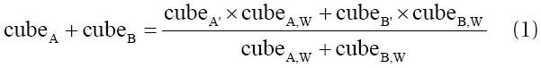
when cube_A,W > 0 or cube_B,W > 0. Here the operation is done pixel by pixel. cube_A' and cube_B' are extended cubes from the original data cubes to a volume enough for the combined cube. cube_A,W and cube_B,W are template cubes containing the weighting information (Fig. 12).

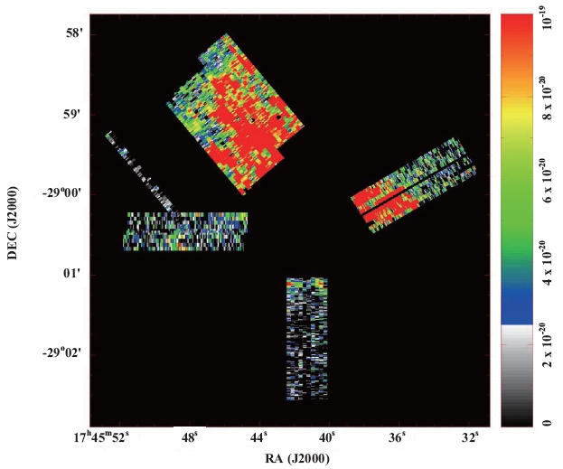
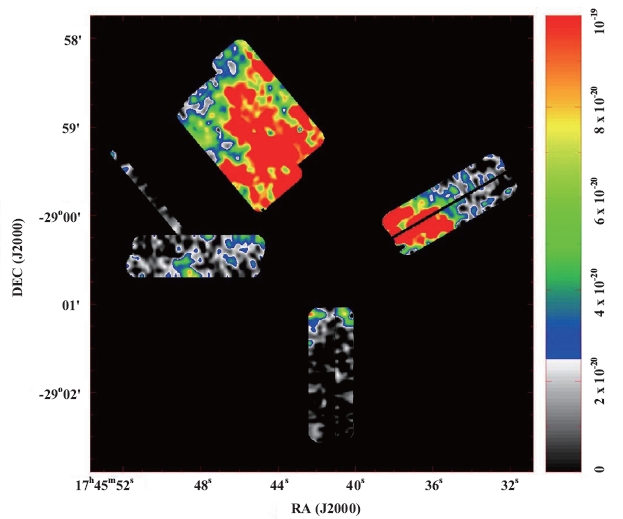
We present results from the mosaicking process in Fig. 13. Throughout all the following stages thereafter for scientific discussions in Lee et al. (2008), we only need this unified cube for the entire region for all kind of analyses such as extracting spectrum, velocity channel maps,

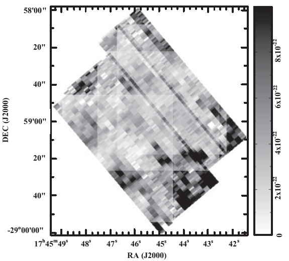
position-velocity diagrams, and direct comparison with radio data. A smoothed version of the global cube, which is convolved with a Gaussian of FWHM = 3 arcsec and has a higher S/N ratio, is also presented in Fig. 14.

Integral field spectroscopy is a powerful observational technic providing higher efficiency and accuracy. In addition to the ability of getting 3D information over the field of view in a single exposure, no light loss through a slit or an aperture keeps the highest throughput of the instrument. The simultaneously obtained 3D data enables reliable calibration both over the field of view and over the wavelength range since there is no time variation between data points in the cube.

Applications using integral field spectrographs have been mostly limited to observations of low dispersion spectrum from small targets such as interacting galaxies. To cover a large field of view with decently high spatial and spectral resolutions, a very long pseudo-slit optics and a very large detector, which are technically difficult and not cost effective, are needed. Scanning observations using long-slit echelle spectrographs are practical choice for this kind of applications although they are less efficient in observing time and less reliable for calibration between slit exposures.

Three-dimensional data, especially at a high velocity resolution, require new methods for data reduction and analysis. In this paper, we introduced one practical approach utilizing a well established tool, MIRIAD, which has been used for years in the field of radio astronomy and is equipped with a number of powerful functions for exploring the spatial-velocity space of 3D data. Our sample application is a survey for a large region with various configurations in the slit position and angle, which must be a complex enough case to test the general capability of the tool. The flexibility and generality of MIRIAD enables us to organize and handle such complicated data cubes. This type of 3D survey would be useful for studies on dynamical structure of large extended objects like supernova remnants and planetary nebulae.

First half of this paper is dedicated to a guideline on the data reduction for long-slit IR spectroscopy. To recover diffuse emission features of extended objects from such contaminations as background radiation, bad pixels, telluric OH lines, and stellar continuum spectra, careful implementation of image processing in a proper sequence is required. We suggested a number of IRAF tools for this process as well as some spectroscopy and geometry tools for image-distortion correction and wavelength calibration.