We developed a photometric pipeline to be used for a wide field survey. This pipeline employs the difference image analysis (DIA) method appropriate for the photometry of star dense field such as the Galactic bulge. To verify the performance of pipeline, the observed dataset of the open cluster M11 was re-processed. One hundred seventy eight variable stars were newly discovered by analyzing the light curves of which photometric accuracy was improved through the DIA.The total number of variable stars in the M11 observation region is 335, including 157 variable stars discovered by previous studies. We present the catalogue and light curves for the 178 variable stars. This study shows that the photometric pipeline using the DIA is very useful in the detection of variable stars in a cluster.
Since Mayor & Queloz (1995) discovered an extrasolar planet orbiting a star similar to the Sun for the first time, about 490 planets have been discovered by various observation methods until early September, 2010 (Schneider 2010). Because the study of extrasolar planets provides a clue to the fundamental questions such as the formation of our solar system and existence of alien life,the research is recently accelerated through long-term projects to use in both ground and space telescopes (Seager & Deming 2010). For the purpose of discovering terrestrial planets in habitable zone, Korea Astronomy and Space Science Institute is developing an extraterrestrial planet searching system (Korea Microlensing Telescope Network; KMTNet) that observes and analyzes a specific region of 4o × 4o in the direction of the Galactic bulge at every 10 minutes based on the microlensing phenomena.Since the density of the stars is very high in the main observation region of this project, a photometric measurement method appropriate for the high dense region is required and the technology to process huge amount of data is necessary as well as close attention in dealing with the data.
One of the photometric engines used for the high dense region including the microlensing experiment is DoPhot that was developed by Mateo & Schechter (1989). In this method, the point spread functions (PSFs) are obtained using isolated stars of which PSFs are well defined,and then the magnitudes of the individual stars are determined by optimizing the PSFs to the observed data. For the most of the early studies for microlensing experiments and dense region observations, several versions of modified DoPhot code were used for their specific objectives (Schechter et al. 1993). However, the photometric results may amplify the photometric error or even give totally different results because of the inaccurate PSFs by the change of seeing condition in the observed region and the blending effect of faint stars. To supplement such drawbacks found in the photometric measurements of dense region, difference image analysis (DIA) method was introduced and applied in many experiments (Crotts 1992, Phillips & Davis 1995, Tomaney & Crotts 1996, Alard & Lupton 1998, Reiss et al. 1998). In this method, the convolution kernel that represents the difference of the PSFs between the reference image and the observed image is obtained and it is applied to the reference image to create a convolved image. Then, a residual image is produced by subtracting the convolved image from the observed image. By applying aperture photometry or PSF photometry to the residual image, photometric measurements for all stars can be obtained. Because non-variable stars are all eliminated, variable stars are appeared to be bright or faint in the residual image. In particular, the blending effect due to the high density of the adjacent stars is also eliminated and thus the photometric performance is excellent.Due to the benefit of DIA, it is very useful to detect variable stars in the high dense regions.
In this article, we describe the photometric pipeline that was established to efficiently detect variable stars in dense region. The improved photometric accuracy and the variable star detection efficiency of the novel photometric method are discussed by the comparing the observation data of the open cluster M11, re-processed by the photometric pipeline with the previous results of Koo et al. (2007) and Messina et al. (2010).
This is an Open Access article distributed under the terms of the Creative Commons Attribution Non-Commercial License (http://creativecommons.org/licenses/by-nc/3.0/) which permits unrestricted non-commercial use, distribution, and reproduction in any medium, provided the original work is properly cited.
The residual image (Diff) is obtained by subtracting the convolved image from the observed image (Obs). The convolved image is prepared by convolution of the reference image (Ref) and the convolution kernel (Ker) and adding the background (Bgr), as shown in Eq. (1):

where x and y represent the pixel coordinates of the observed region and u and v represent the two-dimensional arrangement defined by dividing the observed region into a certain size. If there is no difference between the reference image and the observed image, the residual image is flat since the two images have all the same values. On the contrary, if there is a variable star in the observed image, it is readily detected because the star is found to be bright or faint in the residual image. Taking advantage of this, the DIA is frequently used in the variable star detection in dense region through time series analysis. It shows an excellent result as it is also applied to the large data processing of the recent microlensing experiments by optical gravitational lensing experiment (OGLE; Udalski 2003) and microlensing observations in astrophysics (MOA; Bond et al. 2001) research groups.
One of the significant elements of the DIA is to calculate the kernel between the reference image and the observed image rapidly and accurately. In this regard, some of the researchers (Phillips & Davis 1995, Tomaney & Crotts 1996, Reiss et al. 1998, Alcock et al. 1999) suggested Eq. (2) as the PSF matching algorithm (PSFM) for the calculation of the convolution kernel:
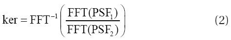
where FFT represents fast Fourier transform and the kernel is defined as the inverse FFT of dividing two FFTs of the PSFs. Since the Fourier Transform is included in the calculation process, the encoding is complex. Although a number of stars that have sufficient S/N ratio and that are sufficiently bright and separated from each other should be selected from the time series observation image,such conditions are hardly satisfied in the images from actually dense regions. On the other hand, Alard & Lupton (1998), Alard (2000), Wozniak (2000) and Wozniak et al. (2001) suggested optimal image subtraction (OIS) method to solve these problems. In this method, the convolution kernel is defined by multiplying the pre-defined Gaussian functions such as σ = 0.78,1.35,2.34 to the polynomial coefficients and adding the background change in the form of polynomials. The defined convolution kernel is shown in Eq. (3):
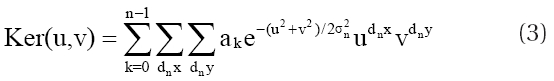
where n, σn, ak, dnx, and dny represent the number of Gaussian functions composing the kernel, the predefined Gaussian function, the polynomial coefficient and the orders of the polynomials, respectively. As shown in Eq. (1), the convolution of Ker with Ref and the combination with Bgr give the convolved image similar to Obs. By assuming the difference between the convolved image and the Obs is nearly zero, a linear equation that satisfies the condition can be constituted. Finally the convolution kernel is obtained by solving the linear equation using LU decomposition, and it is more convenient than PSFM including calculation in the complex Fourier Space.
3. CONSTITUTION OF THE PHOTOMETRIC PIPELINE
We used OIS method to constitute the photometric pipeline since it is more convenient for the encoding and batch calculation than PSFM. The currently available OIS codes are image subtraction package ISIS code developed by Alard & Lupton (1998) and DIA code developed by Wozniak (2000) both of which stability has been verified as they are applied to the photometric pipelines of various observation projects. Although both codes were prepared using ANSI C language and can be used without limitation as open codes, we used DIA code in constituting our photometric pipeline by modifying it because DIA code is more intuitive and prepared more systematically than ISIS code. The photometric pipeline that we developed is described in detail in Lee et al. (2009) and the core features are summarized here.
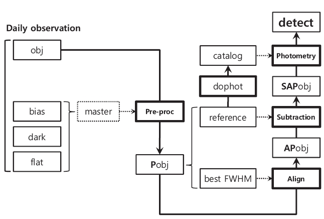
The key steps to constitute the photometric pipeline are pre-processing, image alignment, image subtraction, photometry, and calibration. For the efficient processing of the individual steps, well-known data processing packages such as DIA, image reduction and analysis facility (IRAF), WCSTools and DoPhot and other codes written by ANSI C language were used. In addition, for the convenience of parameter input and output and version control, the entire pipeline constitution was performed by using PERL script that has excellent capability for character string input and output. Fig. 1 shows the schematic diagram of the individual stages of the photometric pipeline constitution.
The master images for pre-processing are combined by running the IRAF tasks such as ZEROCOMBINE,
DARKCOMBINE and FLATCOMBINE in the PERL script, and then the observed images are pre-processed using the CCDPROC task. In the case where the observation is performed in multiple observatories, the identifiers to distinguish each observatory are used and pre-defined parameters are applied for pre-processing.
For the observed images that underwent the pre-processing, the pixel coordinate is transformed so that it can be matched with that of the reference image, using the programs written in ANSI C code such as CROSS, segmented image undergoes star finding (SFIND) and XYMATCH and the IRAF tasks such as GEOMAP and GEOTRAN. The first step of alignment is to create the reference image. While this step is not required if there is already the reference image or additional measurement was not carried out, the first step to produce the reference image should be taken when there is no reference image. From the observed images, a small part of 128 × 128 pixels is taken and star searching is performed within the region. A total of 100 images are selected according to the order of the number of stars found and then 50 of them are re-selected in the order of low background. Finally, 20 images were again screened in the order of good seeing and then the good seeing images were prepared as the reference image after the coordinate conversion and combining. From the Mt. Lemmon and the MOA data processing, the best results were obtained when we use 20 good seeing images.
After obtaining the combined reference image and the best seeing image from good seeing images, all of observed images are moved to the working directory to carry out the alignment procedures with the best seeing image. Each of the observed images is cross correlated with the best seeing image and the approximate offsets of the x- and y- coordinates are calculated. Referring to the value, a certain size of segmented image from the whole image is taken and saved. The SFIND procedure for more precise coordinate transformation and the procedure to find the list of the stars located at the same place with that of the stars found in the reference image is followed (XYMATCH). After these procedures are finished, the list of the overlapped stars is saved and ready to calculate the precise coordinate transformation coefficients of the two lists (GEOMAP). Based on this transformation equation, the pixel coordinates of the observed images are transformed (GEOTRAN) to finish the image alignment stage.
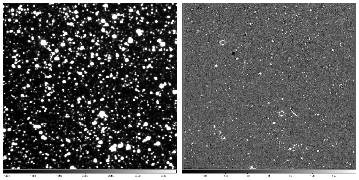
We modified the DIA code that was developed by Wozniak(2000) to use it for the image subtraction engine. As described in Section 2, the convolution kernel is obtained through OIS using the observed images and the reference image. Fig. 2 illustrates an example of the reference image(left) and the residual image (right). As shown in the Figure, the non-variable stars have the value close to zero in the residual image, while the variable stars show white or black spots as they become brighter or fainter so that they can be easily identified even with the naked eyes. The locations of the saturated region in the reference image are masked so that they may not be included in the calculation of the convolution kernel and they are shown gray in the residual image.
3.4 Photometry and Calibration
The magnitude of the stars in the residual image should be calibrated by adding the residual flux and the original flux. Since the residual image is obtained through the image subtraction, the original flux of the individual stars is not included. Hence, when converting the residual flux change into the magnitude, the original flux should be included using the reference image. Also, since the residual image shows almost flat in contrast to general images and only the stars that have undergone the light variation remain in the brighter or fainter state, it is difficult to de-
termine the central coordinates of all the stars accurately. To solve this problem, we made the pixel coordinate list of all of stars using the reference image and applied the star list to all the residual images for the photometry. DoPhot is used for star searching and photometry in the reference image. The magnitude of each star is determined by combining the original flux to the flux change at each coordinate using Eq. (4):
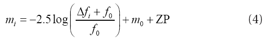
where mi represents the instrumental magnitude, Δfi the flux measured in the residual image, f0 the flux measured in the reference image, m0 is the instrumental magnitude determined by DoPhot, and ZP is the instrumental magnitude zero point approximately calibrated to the standard magnitude system.
4. DETECTION AND CLASSIFICATION OF VARIABLE STARS
From the observed data of open cluster M11 by Koo et al. (2007) at the Mt. Lemmon Observatory for 18 days from June 6 to June 23, 2004, re-processing was carried out with a total of 371 observed images obtained at the 600 seconds of exposure in V-band. The photometric pipeline is a script file containing about 1,600 lines and this file is modified so that it could allow parameter setting at each of the processing stages and steps. Considering that the central part of M11 is heavily saturated, each of the 2 K × 2 K observed images were divided into sixteen 512 × 512 segmented images for the processing. As described previously, the S/N ratio of the reference image is much improved when compared with the observed image if the reference image is produced by combining with images of good quality. Thus, the number of stars obtained by the DoPhot photometry of the reference image is larger than that obtained from observed images. The number of stars in the reference image found by controlling the threshold was about 50,000, among which 32,000 are also included in the list of stars found by Koo et al. (2007). The total CPU time for the data processing was about one day when 3 GHz single core with 8 GB memory was used.
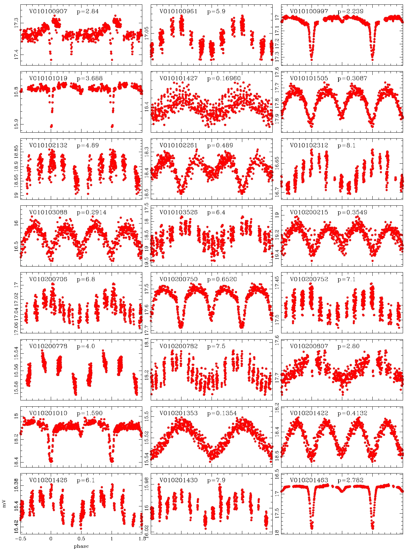
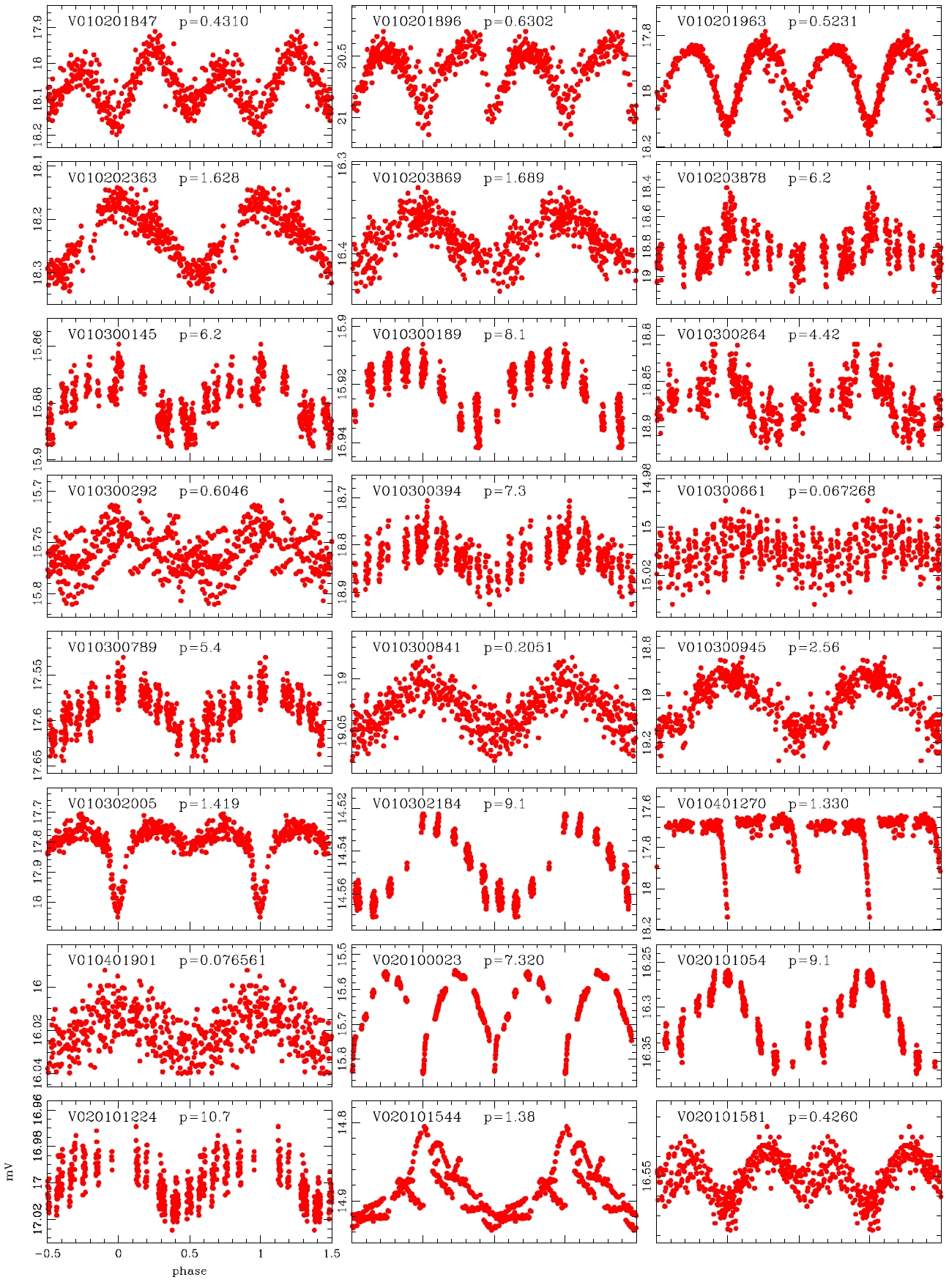
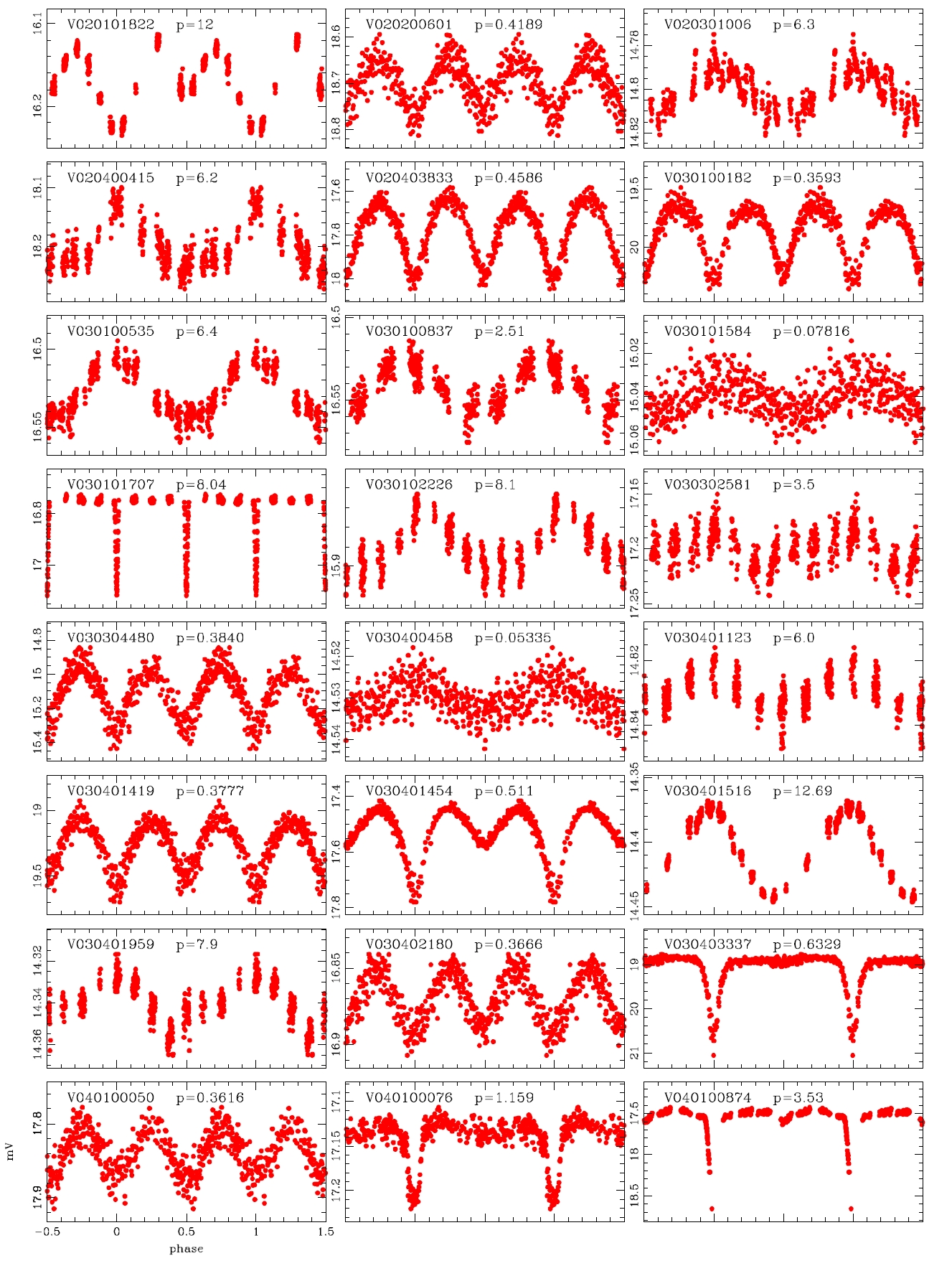
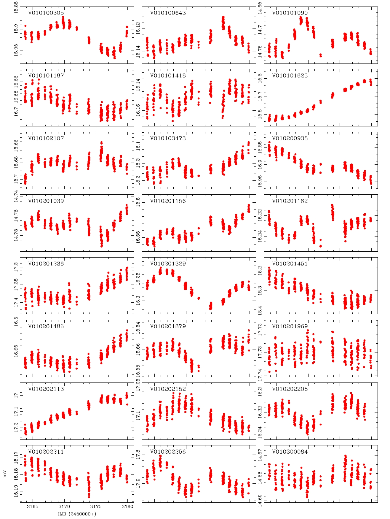
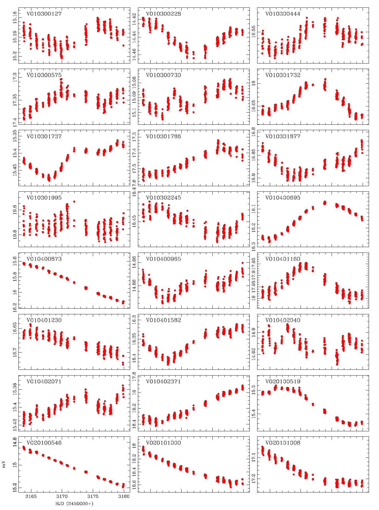
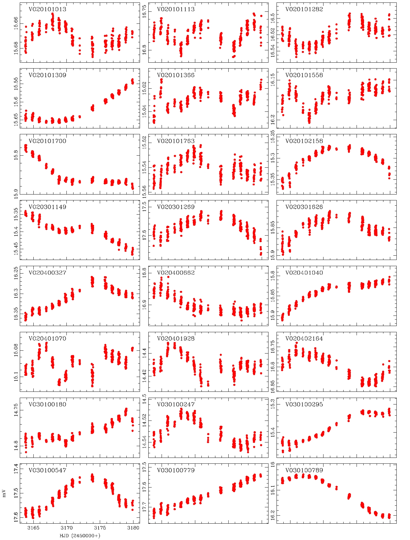
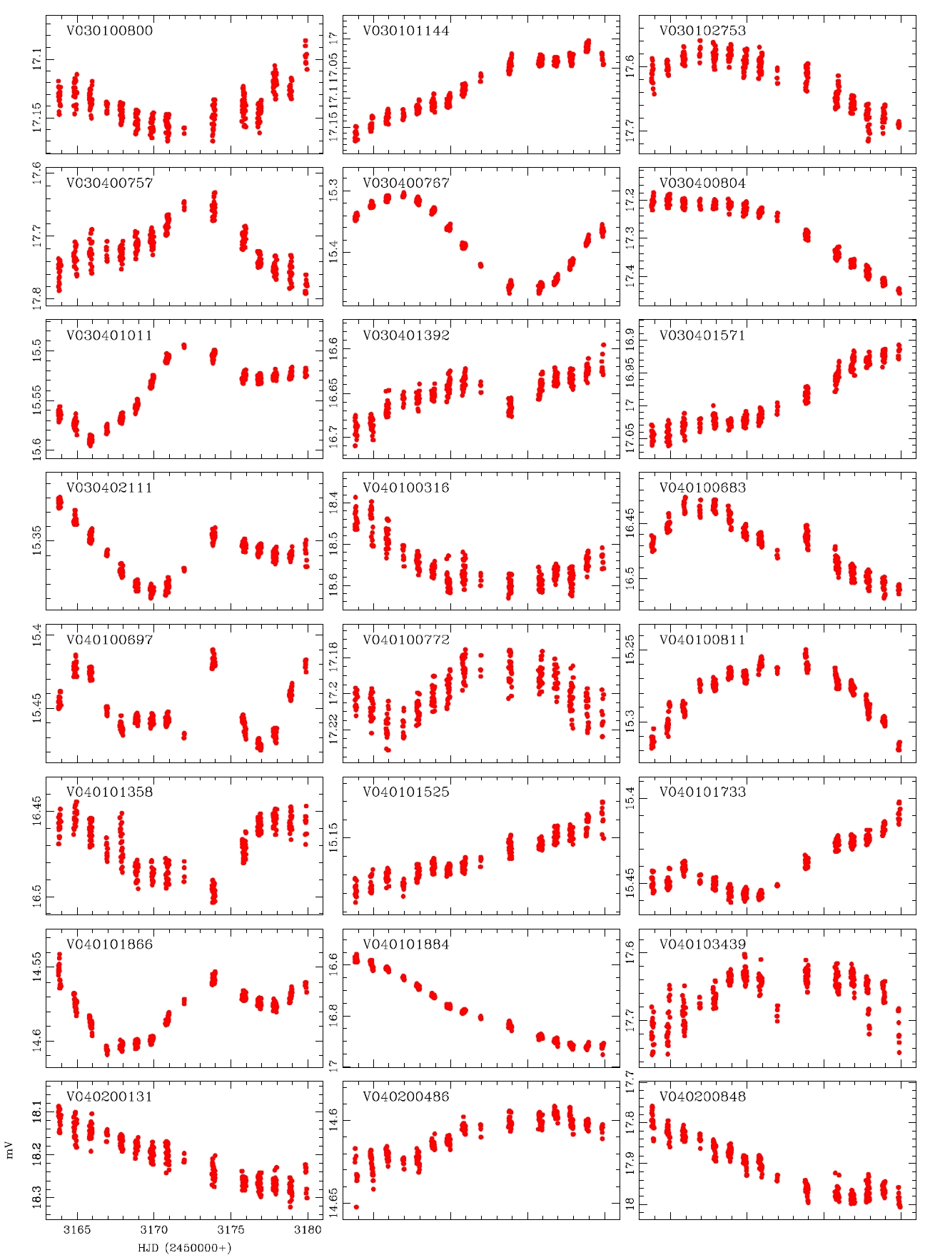
Koo et al. (2007) conducted the data processing by applying the PSF photometry and ensemble normalization technique. They summarized totally 82 variable stars including the 39 variable stars discovered by Hargis et al. (2005) and 43 variable stars discovered newly. On the other hand, Messina et al. (2010) examined the power spectra of the individual light curves using the photometric data of Koo et al. (2007) and detected 75 variable stars additionally. We processed the same observation data and obtained about 50,000 light curves and conducted visual inspection to detect the variable stars. For the light curves in which light variation was found, the variation period was determined with period determination program based on the Lomb-Scagle method (Press et al. 2007) and the power spectrum analysis. Considering that the total observation period was 18 days, the light variation period was determined within 13 days. The variable stars of which the period was longer than 13 days or of which periodicity was not observed were classified as undetermined system. As a result, a total of 178 variable stars were newly discovered including 76 periodic variable stars and 102 undetermined variable stars. Thus, currently, the total number of variable stars discovered in M11 is 335, including 82 summarized by Koo et al. (2007), 75 discovered by Messina et al. (2010) and 178 newly discovered in this study.
The light variation shape of the W UMa type eclipsing binary stars, being similar to a sine curve, is very similar to that of the δ Sct and RR Lyr type pulsating variable stars. Thus, it is very difficult to identify the accurate type of variable stars based only on their single filter light curves. Hence at least two filters should be employed to see the change of the amplitude at different wavelength bands for accurate classification (Jin et al. 2003, 2004). Because the data that we processed in this study was observed only using the V-band, the change in the amplitude depending on the wavelength bands could not be found. Therefore, the variable stars that were clearly differentiated in terms of the slope at the maximum light or the shape of the curve at the minimum light were classified as the W UMa type. The star which did not show the feature of W UMa type or of which variation period was shorter than 0.3 day according to the definition of Breger (1979) was classified as the δ Sct type.
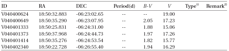
According to the criteria, we analyzed the variation periods and types of the 335 variable stars that have been discovered until now based on the light curves, and found that 29 of these were mischaracterized in the previous studies. Table 1 summarizes the result of the newly discovered 178 stars and re-defined 29 stars. The number of W UMa, δ Sct, Algol and β Lyr type variable stars were 17, 11, 13 and 7, respectively.
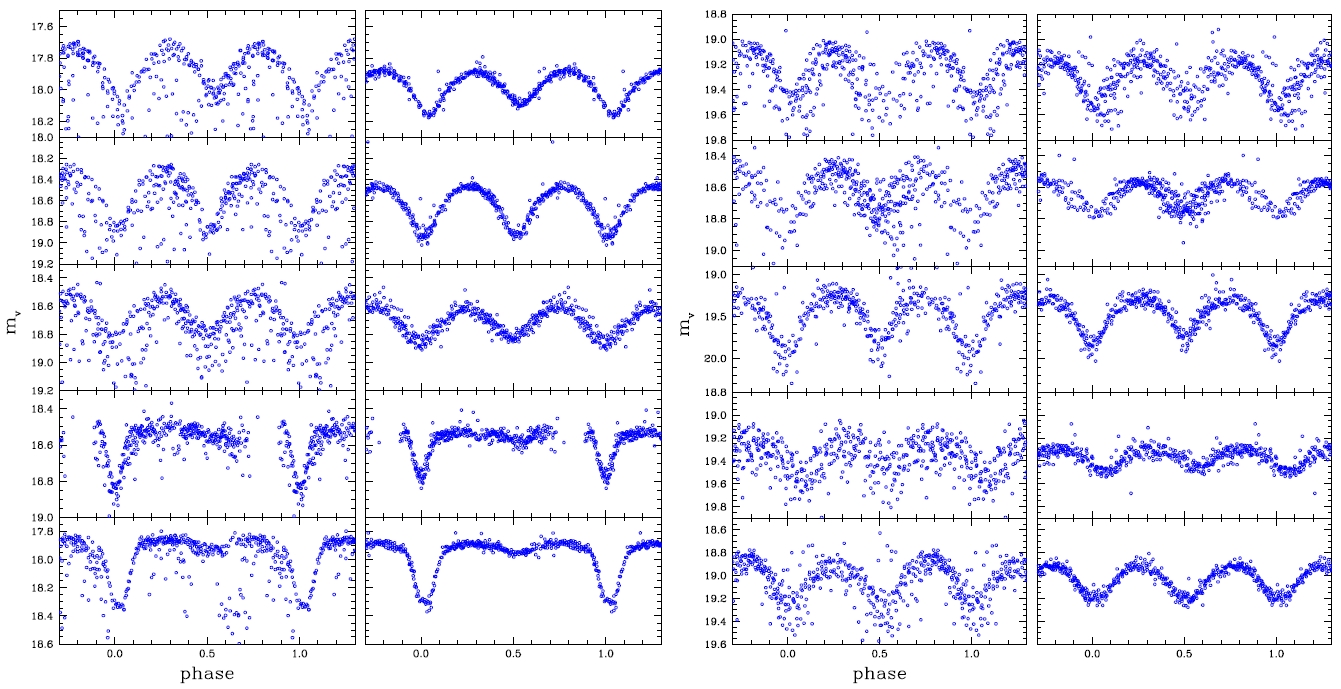
The reasons why the discovery and classification were improved when compared with those of the previous studies include the data processing characteristics of the DIA. Particularly, elimination of the blending effect and the background brought improved photometric accuracy which gave well-defined light curves. To compare this effect, among the list of the variable stars presented by Koo et al. (2007), the light curves of which blending effect is large and faint were compared in Fig. 3. The Figure shows that the photometric accuracy of the light curve was better when the DIA method was applied than the PSF photometric method. Thus, the result suggests that the long-term observation with the DIA and multi filters are very essential in the discovery and classification of variable stars in dense region.
We developed a photometric pipeline based on the DIA for the improvement of the photometric accuracy in the crowded field such as microlensing experiment. The observation data of the open cluster M11 with relatively high stellar density was re-processed using the photometric pipeline we developed. A list of about 50,000 stars was generated and the light curves of the individual stars were obtained from the DIA. The photometric accuracy of the light curves was greatly improved when compared with that of the previous studies in which PSF photometry was conducted. 178 variable stars were newly discovered from the photometric results of this study. The light curves of the 335 variable stars discovered so far were an
[Table 1.] Catalogue of variable stars discovered in open cluster M11.
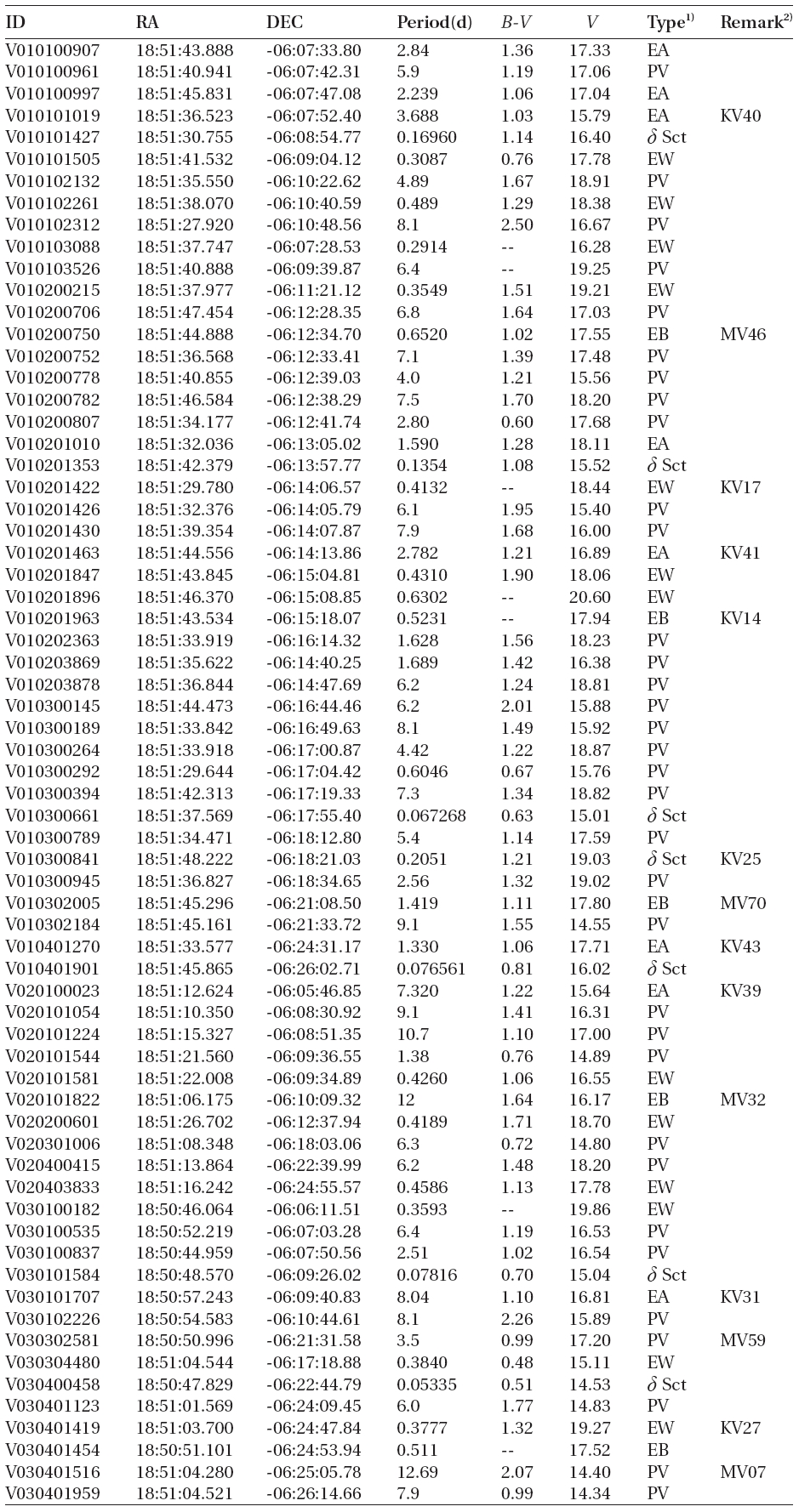
Catalogue of variable stars discovered in open cluster M11.
(Continued)
(Continued)

1)EA, EB, EW, δ Sct, PV represent Algol, β Lyr, W Uma, δ Scuti, and periodic variable, respectively.
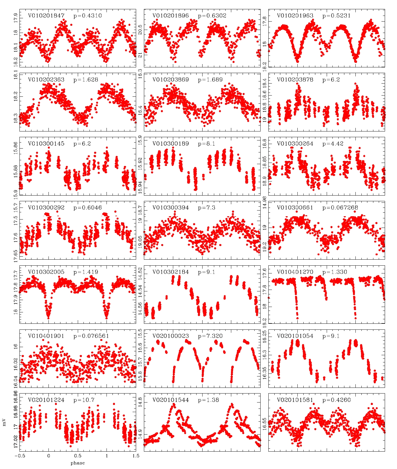
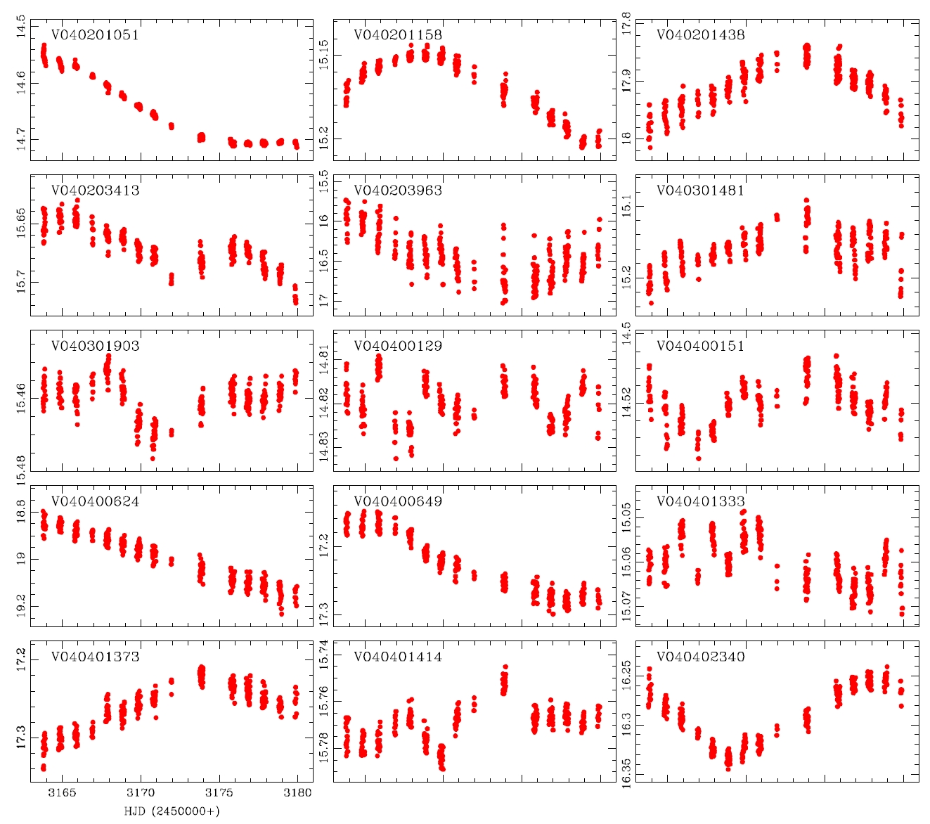
alyzed and the variable periods and types were newly determined for 207 light curves, as summarized in Table 1.The information of the 29 variable stars mis-determined in the previous studies is included in Table 1.The number of W UMa, δ Sct, Algol and β Lyr type variable stars newly determined in this study were 17, 11, 13 and 7, respectively, but 159 stars were not determined yet. Fig. 4 shows the light curves of the variable stars that were newly defined through this study.
While the accurate light curves could not be able to be obtained by the photometric method using the conventional PSF photometry because of the problems such as blending effect and low S/N ratio, well-defined light curves were obtained by the DIA. This is because of the characteristics of the DIA technique which is elimination of blending effect and background. In addition, for accurate classification of variable stars, the long baseline of the light variation using at least two filters are essential. The developed photometric pipeline is currently used in the microlensing experiment and the study of variable star searching in crowded field. Also it will be used in the data processing of the extraterrestrial planet searching system (KMTNet) that is currently developed by Korea Astronomy and Space Science Institute. For this, it is necessary to improve the current code to be able to do multi-process to enhance the processing speed, and the
light variation detection algorithm to discover and classify variable stars.