The positioning method using global positioning system(GPS) is developing continuously and the information provided is very accurate and precise currently. The most widely known method for the GPS high-accuracy data processing is the relative positioning method, which determines the precise position using the relative difference between the reference station and the user. The relative positioning method can achieve a very high level of positional accuracy by eliminating the clock error of the satellite and the receiver, that biggest positional error, through the difference between the satellite and the receiver. However, this method requires the observation information or the correctional information generated by the reference station and the accuracy of the user’s position is very closely correlated with the reference station. Additionally, there are a few constraints as the baseline distance between the reference station and the user is increased. First, if the baseline distance is longer than 2,000 km, the accuracy of the user’s position is decreased or the positioning becomes impossible because of the number of common satellites is insufficient. Second, the ionospheric and tropospheric delay can be neglected when the baseline distance is short. However, if the baseline distance is longer than 10 km, the atmospheric error must be taken into account for the estimation or the positioning should be performed by compensating the error through an observation model. The position of a moving object can be determined in the accuracy of approximately 1 m within range of the baseline distance of 10 km when the relative positioning method is used, and in the accuracy of approximately several centimeters in the case of static survey (Farwell et al. 1999, Mendes 1999).Park et al. (2003) used the relative positioning method for general survey and reported the analytical result that the positioning error was less than 6 cm. Additionally, Choi et al. (2009) showed that the positional error of each element was less than 2 cm on a short baseline.
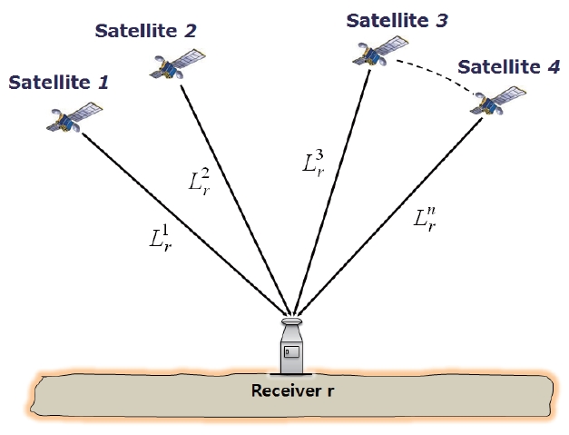
As described previously, one of the biggest drawbacks of relative positioning is that the reference station information is necessary. The method that was developed to compensate the drawback is the precise point positioning(PPP) method. PPP was developed by the US Jet Propulsion Laboratory (JPL) in the late 1990’s. The most representative software is GIPSY/OASIS II (Heroux & Kouba 1995). In this method, the position of the receiver is calculated in a high accuracy without referring to a specific reference station as shown in Fig. 1 (Zumberge et al. 1997).
For PPP to maintain the positioning performance similar to that of the relative positioning method, it requires very precise satellite orbit and clock information determined in advance by the International GNSS Service (IGS) observation network. Currently, there are approximately 430 active international reference stations in the IGS observation network. Among them, approximately 100 reference stations whose position and clock information are stable are finally selected to precisely calculate the satellite and receiver clock error as well as the satellite orbit. Additionally, the Earth’s tide modeling information is needed including the crust, ocean and polar tide.
PPP employs the post-processed IGS final output to calculate highly precise position. Since approximately two weeks are needed in average to generate the IGS final output, PPP has been recognized as a post-processing method. However, an international campaign has been conducted to generate real-time satellite orbit and clock information since 2008, the recent studies are actively carried out on the PPP method once again.
As explained previously, in this study, we developed
the PPP data processing method using the GPS dual frequency data to compensate the drawback of relative positioning,and compared the result with the precise position values calculated by the IGS analysis centers to verify the performance.
The observation information received from GPS satellites is divided into the code phase and the carrier phase. The code is classified into coarse acquisition (C/A) and precise (P) codes, while the carrier phase is classified into L1 (1,575.42 MHz) and L2 (1,227.60 MHz) frequencies.
The GPS signals are affected by many factors on the path coming to the receiver and the ionosphere causes the biggest error. The free electrons in the ionosphere affect the navigation signals having electromagnetic properties. Signal delay is caused in the GPS code phase by the refraction as the signal passes through the ionosphere whereas signal advance is cause in the carrier phase.
Since the ionosphere is the largest error factor in the GPS data processing, the effect of the ionosphere needs to be reduced or eliminated. Generally, the dual frequency GPS data is used to eliminate the effect of the ionosphere. The ionospheric error can be eliminated by performing the data processing through the linear combination of two carrier phases as in the following Eq. (1) (Hofmann-Wellenhof et al. 2008):

where
The observation information from which the ionospheric effect is eliminated by the linear combination in Eq. (1) is re-expressed as Eq. (2) (Musman et al. 1998, Kouba & Heroux 2001):

where
Additionally, the effect of the earth’s crust, ocean and polar tide as well as the earth rotation parameters should be considered in the PPP data processing. Moreover, the wave front of the GPS signals that is circularly deflected to the right side is affected by the relative motion of the satellite and the receiver, which is called phase windup. This should be also applied to the data processing.
2.1 Estimation of the Tropospheric Delay Error
Estimation of the tropospheric error is very important in the PPP data processing. The troposphere actually affects the position element error of the receiver, especially the upward direction of the receiver. The calculation of the total tropospheric delay is expressed as Eq. (3):

where
In this study, to estimate the ZHD, we applied the Saastamoinen model in the following Eq. (4):

Determination of
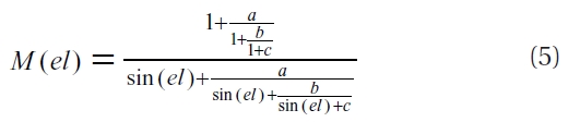
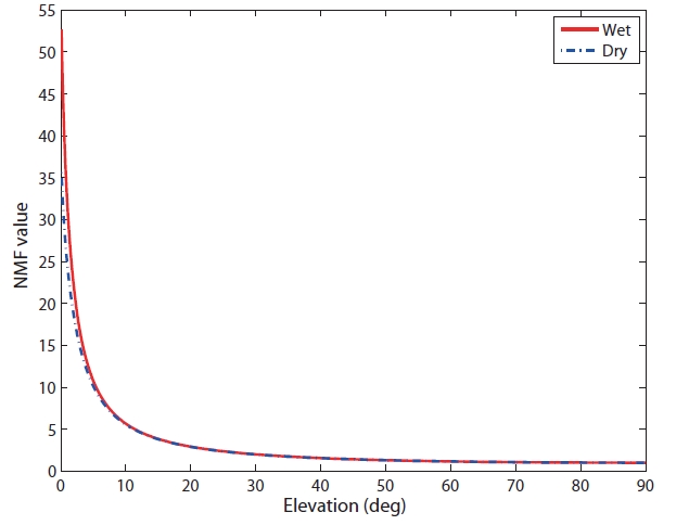
NMF, the model based on geological latitude change (15 degree interval), calculates the coefficients (a, b and c) considering the mean sea level change as well as the temperature and relative humidity. Fig. 2 shows variations of the dry and wet NMF values as a function of satellite elevation angle.
We employed the extended Kalman filter (EKF) to estimate the position, velocity, the trophospheric delay information (ZTD, gradients) and the state variables of the float ambiguities. Eqs. (6) and (7) shows the update and prediction of the individual state variables (Welch & Bishop 2002):
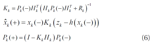
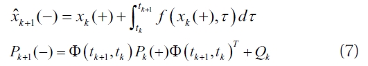
In these equations, the state variables are estimated by a deductive method and an inductive method using the state variable
The finally estimated variable x consists of the variables of

The
The position accuracy is the most fundamental in verifying the PPP performance because the performance of the observation model applied to PPP is directly related with the position accuracy. Dual frequency GPS data is also required to acquire high-accuracy position information.To meet these requirements, there should be the data from a GPS reference station that receives dual frequency information. Thus, in this study, we processed the measurement data received by the Daejeon (DAEJ) IGS reference station for five days between July 1 and July 5 in 2007 to verify the performance of the developed PPP. Table 1 shows the models applied to the data processing procedure.
The values finally estimated following the data processing include the observation time, the position elements of the reference station, the receiver clock error, the tropospheric delay error, the tropospheric gradient information and the float ambiguities.
[Table 1.] Detailed models and settings for PPP.
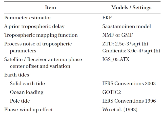
Detailed models and settings for PPP.
3.1 The Applied Observation Model
The preliminary information for the tropospheric signal delay was calculated by applying the Saastamoinen model. The NMF was used as the mapping function. We assumed random walk for the estimation of the tropospheric ZTD and the gradient variables change and set the data processing noise as
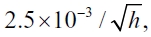
The preliminary information for the tropospheric signal delay was calculated by applying the Saastamoinen model. The NMF was used as the mapping function. We assumed random walk for the estimation of the tropospheric ZTD and the gradient variables change and set the data processing noise as
All the effects of the Earth’s tide were considered: the models suggested at the International Earth Rotation Service (IERS) Conventions 2003 and the IERS Conventions 1996 were applied for the crust and polar tides, and the GOTIC2 (NAO.99b) model for the oceanic tide. The displacement by the Earth’s tide on the navigation coordinate is expressed as Eq. (8):

where Δ
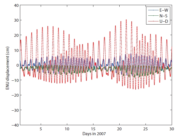
Fig. 3 shows the tidal displacement at the DAEJ IGS reference station for one month in July 2007 calculated by using the tidal models applied to the data processing. The tidal effect in the East-West and North-South directions was within ±5 cm. The displacement in the Up-Down element was relatively large: the maximum displacement was approximately +25 cm and the entire position variation range was ±20 cm. This result shows that the tidal effect may be a great error in the PPP data processing.
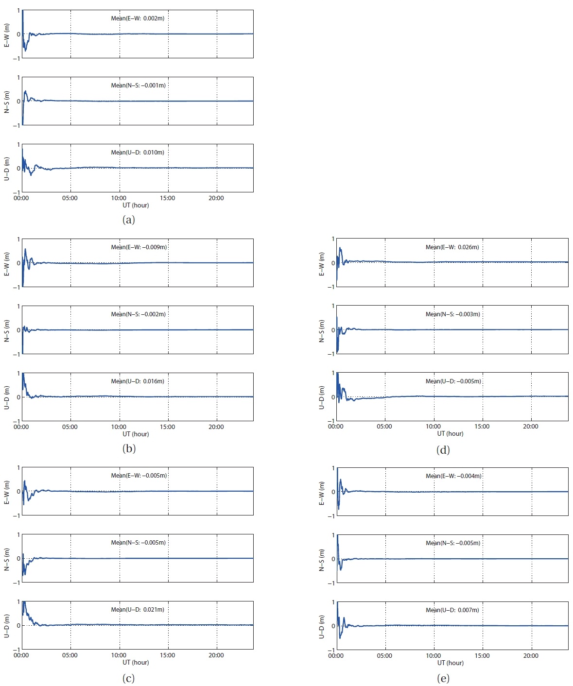
Figs. 4a-e show the results of the data processing in the static mode using the dual frequencies of GPS L1and L2, respectively. The observation data used for the data processing was received at the DAEJ IGS site. The reference station position information was estimated epoch-by-epoch, that is, in a 30 second interval. The data processing was performed each day. The result was compared with the IGS05 reference coordinate provided by the IGS analysis center to verify the processed result. We showed the results generated in this study with reference to the reference station position information (referring to zero) produced by integrating the results from the IGS analysis centers.
Fig. 4a shows the processing result of the GPS data on July 1. The mean value of the reference station positional error was 0.2 cm in the East-West direction, -0.1 cm in the North-South direction and 1.0 cm in the Up-Down direction within the confidence level of 95%. Fig. 4b shows the
processing result of the GPS observation data on July 2. The mean value of the reference station positional error was -0.9 cm in the East-West direction, -0.2 cm in the North-South direction and 1.6 cm in the Up-Down direction. Similarly, Fig. 4c shows the processing result of the GPS data on July 3. The mean value of the reference station positional error was -0.5 cm in both the East-West direction and North-South direction, and 2.1 cm in the Up-Down direction.
The position error in the Up-Down direction was great between July 1 and July 3, while the position error in the East-West direction was greater than that of the North-South direction and Up-Down direction in the data processing result on July 4, as shown in Fig. 4d. Finally, Fig. 4e shows the processing result of the GPS data on July 5. The position errors in the East-West direction and North-South direction were -0.4 cm and -0.5 cm, respectively, and that in the Up-Down direction was 0.7 cm.
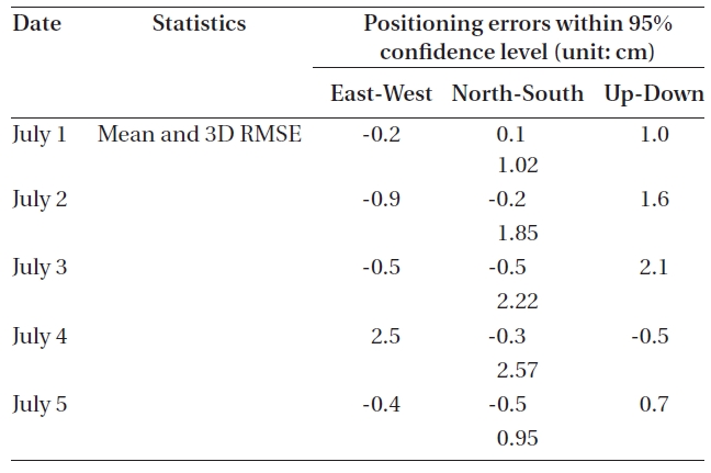
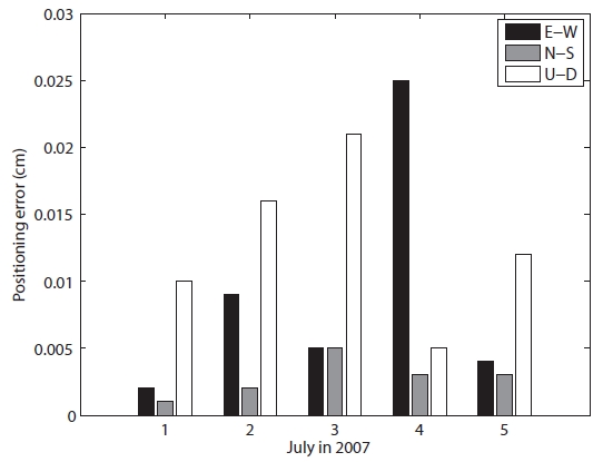
The GPS data for a total of five days was processed by the developed PPP method and the statistical values are shown in Table 2. Fig. 5 illustrated the values in bar graphs so that they can be easily understood. Summarizing the data processing result for the five days, the position error in the East-West direction was less than 1 cm in the confidence level of 95%, except the result of July 4. In particular, the position error in the North-South direction was smaller than that of the East-West direction and Up-Down direction. Generally, the Up-Down direction element shows the greatest error in PPP data processing result and the similar property was found in the result of this study. As shown in Fig. 5, the error was greater in the Up-Down direction element in all the data processing result, except the result of July 4. The known cause for such as result includes the geometric arrangement of the GPS satellites and the effect of the tropospheric delay error. Therefore, the result in this study was very accurate when compared with the results provided by the IGS analysis centers since the error for each element was less than 2 cm.
[Table 2.] Mean positioning errors and the RMSE.

Mean positioning errors and the RMSE.
This study was conducted to compensate the drawback of the conventional relative positioning method, showing that the positional accuracy level similar to that of the relative positioning method can be generated only by the GPS receiver. To improve the PPP performance, we applied various measurement models regarding the Earth’s tidal effect and tropospheric delay that affect the GPS signals and employed the EKF for the estimation of the variables including the reference station position, tropospheric information and the float ambiguities. The ionospheric error, which causes the greatest error in the GPS signal, was eliminated through the linear combination of the dual frequency GPS data which are processed on a daily basis. Consequently, we obtained following results by processing the data of DAEJ GPS reference station for five days:
First, the comparison of the PPP data processing result in this study with the results provided by the analysis centers showed that our result was very precise: the error was 0.9 cm and 0.32 cm in the East-West direction and in the North-South direction, respectively, and 1.14 cm in the Up-Down direction within the confidence level of 95%.
Second, in the case of the DAEJ IGS reference station used for the data processing, the position was varied by ±5 cm in the East-West direction and in the North-South direction and by the maximum of 25 cm in the Up-Down direction by the tidal effects of the crust, ocean and poles.
Third, one of the drawbacks of PPP is that it requires the procedure for initial convergence time, and our result also showed that the data processing for 24 hours had the convergence time of approximately one hour in the initial stage. In order to solve this problem, the integer ambiguity needs to be determined rapidly, and the bias of the GPS satellite and the receiver should be considered meanwhile.
The result of this study showed that the high-accuracy positioning service that has been conventionally provided by the relative positioning method can be sufficiently provided through the PPP method in the future.