The interferometric fiber-optic gyroscope (IFOG) is a representative fiber-optic sensor based on the Sagnac effect to measure absolute rotation rates in inertial reference frames [1-2]. IFOGs have many advantages over conventional gyroscopes, such as long life, high reliability, light weight,low cost, and so on. Many useful research results related with IFOGs have been achieved so that the IFOG is now a good prospective candidate for future inertial navigation systems. However, in spite of such positive advances, there are still some difficulties to be overcome to improve IFOG performance.
The thermally induced non-reciprocity of IFOGs has been one of main obstacles to applying them in practical applications.This phenomenon, the so called Shupe effect, yields transient bias drift when a temporarily changing thermal gradient passes through the rotation-sensing fiber coil [3].With the aid of invaluable earlier works, it could be proved that thermal transient non-reciprocity can be considerably reduced by applying a quadrupolar winding pattern to the fiber coil [4-5]. Nonetheless, this does not sufficiently address the problem because there can still be residual drift much larger than steady-state bias stability depending on the degree of imperfection in the thermal design and fabrication of the fiber coil. Quantitative analysis based on a thermal model considering heat conduction and physical stress is essential to identify proper methodologies which can address the imperfection [5-6]. Because thermal characteristics, such as diffusivity and temperature induced change in the effective index of the fiber coil, are critical factors determining the Shupe effect, it is necessary to examine the behavior of the thermal characteristics in detail to further improve the temporal thermal performance. However, all the established studies in analytic modeling of the Shupe effect have been performed with an assumption that thermal characteristics are invariant over temperature changes even though this is not true in the real world. For an accurate analysis of the thermal transient over a wide temperature range, it is indispensible to examine changes in thermal characteristics as a function of the average temperature measured during experiments.
In this study, temperature dependencies of the transient responses are analyzed focusing on changes in the thermal characteristics of the fiber coil at several fiber coil temperatures.The related theory with analytic model is presented in Section 2, experimental methods, analyzed results, and a summary are given in Sections 3, 4, and 5, respectively.
II. THEORY OF THE SHUPE EFFECT WITH ANALYTIC MODEL
Non-reciprocity due to the transient temperature perturbation caused by differences between the coil temperature and ambient temperature,
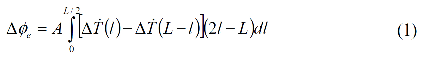
where
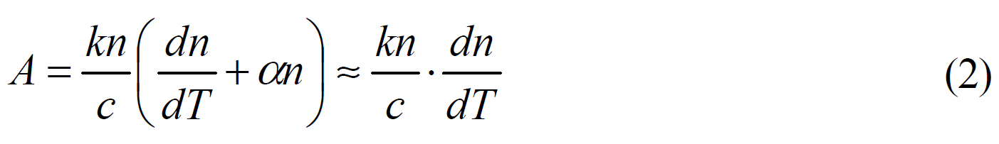
where
For the thermal perturbation applied to the radial direction of the fiber coil with quadrupolar winding pattern,Eq. (1) can be rewritten as a discrete form:
where N is the total layer number,
for a fixed coil geometry. There have been two main methodologies to determine the Δ? ; one is based on the finite element method (FEM) [6], and the other utilizes a numerical calculation with an analytic heat conduction equation [5]. Even though the latter methodology may be less adaptive for correct estimation of
where
where
where
where λ and D are the central wavelength of the light source and the average loop diameter of the fiber, respectively.
Note that the transient rate error due to the thermal perturbation is apparently dependent on
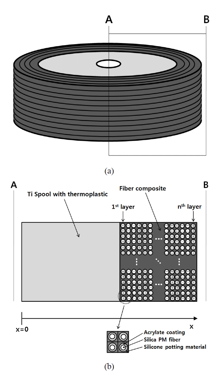
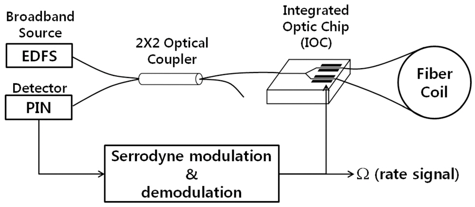
The configuration of IFOG tested in this work is depicted in Fig. 2. The light from a broadband erbium-doped fiber source (EDFS) with a 1550 nm center wavelength is split by a 3-dB optical coupler and then coupled to a fiber which is pigtailed to a LiNbO3 integrated optic chip (IOC)which functions as a TM-mode-rejecting polarizer, a Y-branch 3-dB beam splitter, and an electro-optical phase modulator.A polarization maintaining fiber (PMF) with 80 ㎛ cladding and 155 ㎛ coating diameter, and 1.45 core index is wound in a 40 mm diameter spool for realization of the fiber coil.The total length of the PMF in the coil is about 900 m,and the fiber coil is composed of 60 fiber layers with a quadrupolar winding pattern. After passing through the fiber coil, two counter propagating light beams are interfered at the common input port of the Sagnac loop, and an interference signal is detected at the photo diode. The rate signal is obtained by a closed-loop approach which is based on the serrodyne modulation and demodulation technique. This ensures a linear and stable scale factor [11].
It is very important to check whether other non-reciprocal error sources in addition to the Shupe effect are present in the measured rate bias of IFOG. The presence of any additional non-reciprocal errors causes overestimation in the analysis because they usually cannot be distinguished from the Shupe effect induced errors. The broad spectrum of the utilized EDFS, about 20 nm, reduces not only the nonreciprocal phase error due to back reflections and backscattering in the Sagnac interferometer [12] but also the Kerr
effect [13]. The IOC with a high polarization extinction ratio over 60 dB and birefractive PMF with an h-parameter of less than 10-5 utilized in the fiber coil can suppress the phase error due to the effect of polarization cross-coupling to a considerably lower level [14-15]. The Faraday bias error which is sensitive to magnetic fields is also eliminated by using a magnetic shield case with highly permeable metal[16]. Before the experiment to analyze the Shupe effect, it was confirmed that this configuration has a very small phase error of less than 10-7 radian by testing the IFOG in a static environment without thermal transient perturbation.Because the peak level of the expected phase error due to transient thermal perturbation in this study is larger than an order of 10-6, the configuration can be considered suitable for analyzing the Shupe effect.
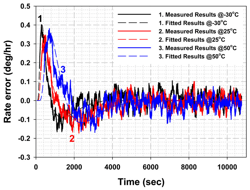
After the preliminary investigation, experiments with the Shupe effect were performed at several surrounding temperatures,namely, -30℃, 25℃, and 50℃, to identify temperature dependence on the critical factors,
For the given coil geometry and
Actually, there may be some overestimation in identifying
the correct values for the thermal characteristics. This is because the experiments and analytic model in this study are not perfect to characterize correct values for
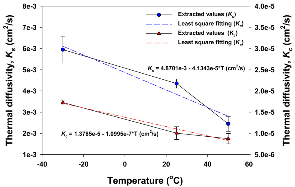
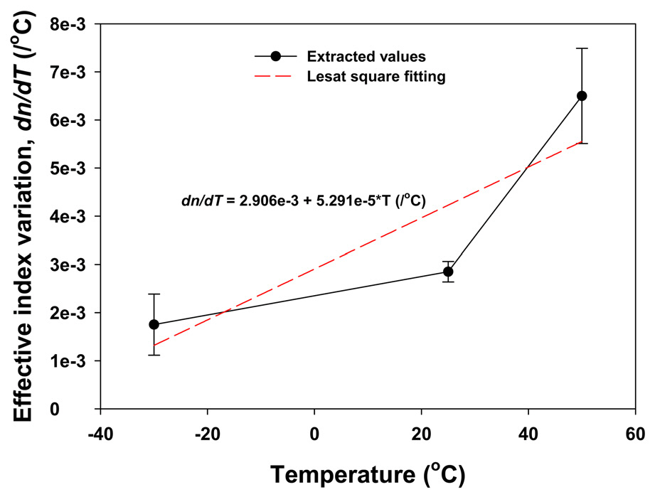
All the extracted critical factors from each experiment are summarized in Figs. 6 and 7. It is possible to confirm two noteworthy tendencies in Figs. 6 and 7. One is that
coefficient which can enhance the stress induced index change as the temperature of the fiber coil is increased [17], these results seem reasonable. Although it is difficult to estimate the correct values for the critical factors by using the thermal characteristics of the constituting material themselves, this fact is sufficient to conclude that the comprehensive thermal characteristics of the fiber coil have the same tendencies as the constituting materials on the temperature changes.The fractional changes in the extracted values can be evaluated effectively by assuming that they comply with linear temperature increase as seen in Figs. 6 and 7. By applying the 1st-order least-square fitting technique to the extracted values, the constant change rates of
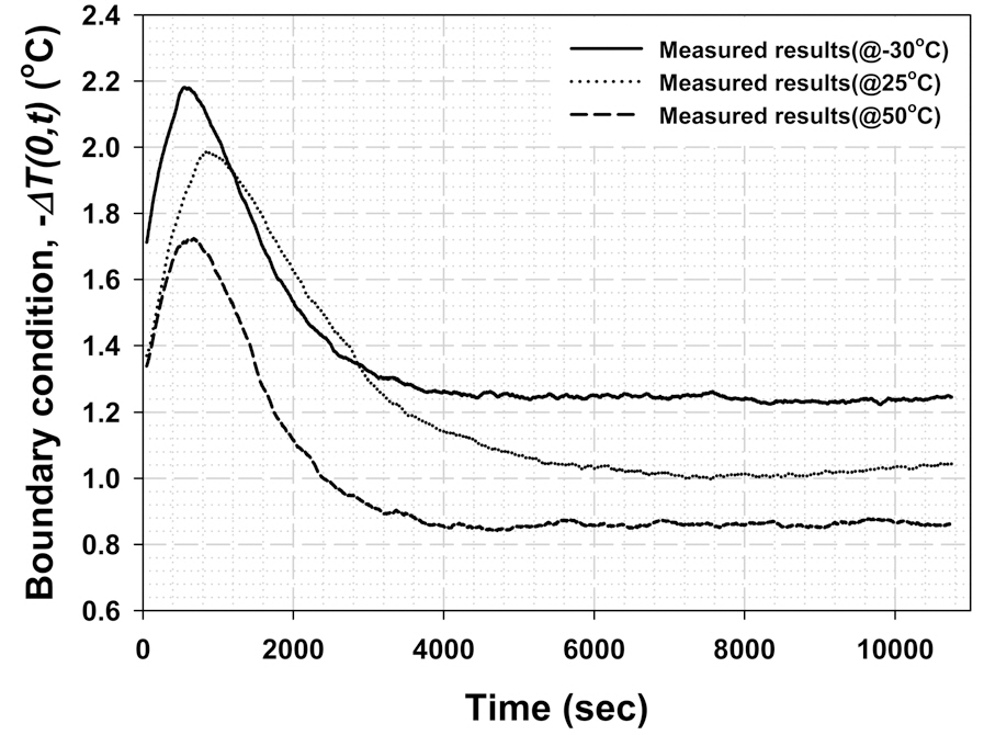
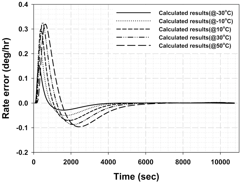
The analyzed simple linear equations from Figs. 6 and 7 are very advantageous when they are utilized in the estimation of the Shupe effect based on the analytic model because they can generate reasonable values on the critical factors at arbitrary temperatures within the considered range.The calculated Shupe effect induced biases for five different temperatures utilizing the extracted linear equations and the analytic model are presented in Fig. 8. The boundary conditions which are necessary for the calculation of the Shupe effect induced biases are assumed to be same as that measured at 25℃. The calculation results in Fig. 8 show that the peak-to-peak quantity and the zero-crossing time of the Shupe effect induced bias increase with increase in the surrounding temperature. These calculation results have a tendency similar to that of the measured results seen in Fig. 4 in the aspect of the broadening of the transience.However, the variant features of the peak-to-peak quantity seen in Fig. 8 do not seem similar to that of Fig.4. The peak-to-peak quantity of the Shupe effect induced bias measured at -30℃ is obviously larger than that of the results measured at higher temperatures of 25℃ and 50℃.These differences between Figs. 4 and 8 are due to the different boundary conditions in the process of estimating
the Shupe effect induced error. Considering that the nominal values of the boundary condition measured at -30℃ are larger than those of the boundary condition measured at 25℃ and 50℃, as seen in Fig. 3, the variant features in the peak-to-peak quantity of the Shupe effect induced bias in Fig. 4 are essentially identical to the features of Fig. 8.
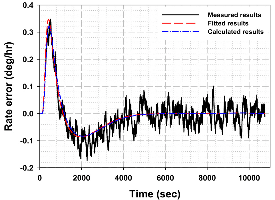
From the results of Figs. 4 and 8, it can be easily confirmed that the variation of the Shupe effect induced error per unit of temperature change is very small relative to the intrinsic outputs in steady-state, which drift and swing within the bounded range of ±0.1 deg/hr. Because the Shupe effect is analyzed based on the measured outputs of IFOG,any measurements for numerous surrounding temperature that do not exhibit distinct variations in the Shupe effect induced error more than the intrinsic bias uncertainty of IFOG can be supernumerary. Because the transient-state is usually inclined to have poorer performance than the steady-state section even when the Shupe effect induced error is not considered, for an accurate analysis, it is more important to achieve good bias repeatability in the transient-state. In this study, it was confirmed by taking repeated measurements at the predetermined surrounding temperatures that bias repeatability in the transient-state is as good as that in the steady-state section. The confirmation of bias performance and the corresponding three temperature points for measurement and analysis in this study are the minimum suitable conditions for analyzing the Shupe effect with the extracted variant equations over the considered range of temperatures.For 25℃, the calculated Shupe effect induced error with the variant equations is presented together with the fitted results based on the analytic model and the measured data in Fig. 9. It can be easily found out that there are negligible differences of less than 0.03 deg/hr between the fitted and calculated Shupe effect induced bias error.
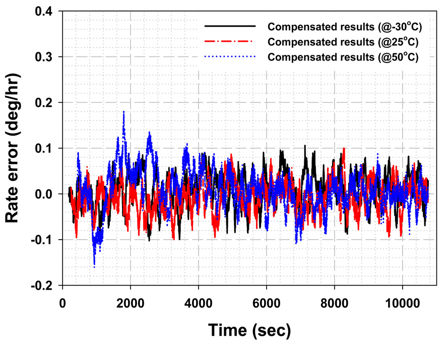
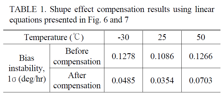
In Table 1, the results of Shupe effect compensation using the linear equations are summarized. The compensation is carried out with only the transient data up to initial 1
[TABLE 1.] Shupe effect compensation results using linearequations presented in Fig. 6 and 7

Shupe effect compensation results using linearequations presented in Fig. 6 and 7
hour of the measured results for 3 hours and the presented values in Table 1 are worst cases of the compensated results. Even though the compensation is not as precise as the results with the extracted values seen in Fig 5, this compensation still considerably improves the bias performance of the IFOG over a wide range of temperatures.
Temperature dependence on the Shupe effect of IFOGs was analyzed in terms of the thermal characteristics of the fiber coil. It was confirmed that thermal characteristics, such as diffusivity and temperature-induced change in the fiber mode index of the fiber coil, were critical factors that determined the Shupe effect of IFOGs. By applying an analytic model with 1-dimensional heat conduction and the geometry of the fiber coil to the measured transient responses of an IFOG, the critical factors were accurately identified. Temperature-induced changes in the critical factors were also analyzed by experiments at three different temperatures,and these factors exhibited variant tendencies to temperature changes. They were confirmed to be essential in compensating the transient effect over a wide range of temperatures.