In-plane switching(IPS) technology imparts to Liquid Crystal Displays(LCDs) many desirable properties such as high contrast ratio, no gamma shift, stable color reproduction,wide viewing angle, and so on. These advantages make in-plane switching technology a strong candidate for high definition(HD) TVs, computer monitors and mobile appliances[1].
Inter-digitated electrodes fabricated on the same substrate are a characteristic structure of IPS-LC Panel, and produce a strong vertical electric field as well as the horizontal one.The coexistence of the vertical and horizontal fields generates a complicated spatial distribution of LC molecules. In this case, only the result of numerical methods conducted by including Berreman’s Q tensor representation can describe the multidimensional director configurations [2, 3]. Once the distribution of directors is given, the intensity transmittance can be obtained by various methods : finite-difference timedomain method [4, 5], beam propagation method[6], reducedorder grating method or a combined method [7-9]. Recently H. J. Cho, et. al. have proposed a simple one-dimensional model for the director distribution in an in-plane switching liquid crystal panel and have calculated the intensity transmittance by using the Jones matrix method [10]. They have reported an excellent agreement between experimental data and computer simulations.
In this paper we report an optical effect recurring in the experimental data of the intensity transmittance through an IPS-LC panel and propose a greatly reduced experimental procedure for characterizing an IPS-LC panel. The new method allows us to save time both in the experiment and computer simulation.
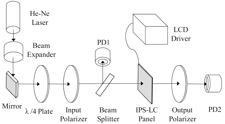
We first measure the light intensities transmitted through an IPS-LC panel by changing the polarization of the input beam and by changing the signal voltage applied to an LC panel. We collect data following the general procedure for the transmitted light intensity[10, 11]. FIG. 1 shows a schematic diagram for the experimental setup. In the experiment, we use a commercial LCD manufactured by LG Display for mobile displays. A beam from a He-Ne laser is first expanded by a beam expander to a diameter of 30 mm and then given circular polarization by a quarter-wave plate. The beam is given linear polarization by an input polarizer before it is incident to the IPS-LC panel. To monitor a possible fluctuation in the input beam, we measure the beam intensity with photo detector PD1. We measure the polarization state of the modulated beam from the LCD with an output polarizer and photo detector PD2. The intensity transmittance is defined by the ratio between the output intensity measured at PD2 to the input intensity measured at PD1. To cancel out the system noise, we normalize the intensity transmittance by the loss factor squared. The loss factor will be discussed later.
Our IPS-LC panel can display 64 gray levels. When we input a two dimensional image of a gray level to the LCD driver, it is converted to a driving voltage and is applied to the LCD panel. We measure the transmitted intensity by changing the input gray level, and the polarization states of the input and output laser beams. For a fixed gray level,we measure the loss factor squared by measuring the maximum and the minimum output intensities for possible combinations of the input polarizer and the output polarizer rotations, and dividing their sum by the input beam intensity.
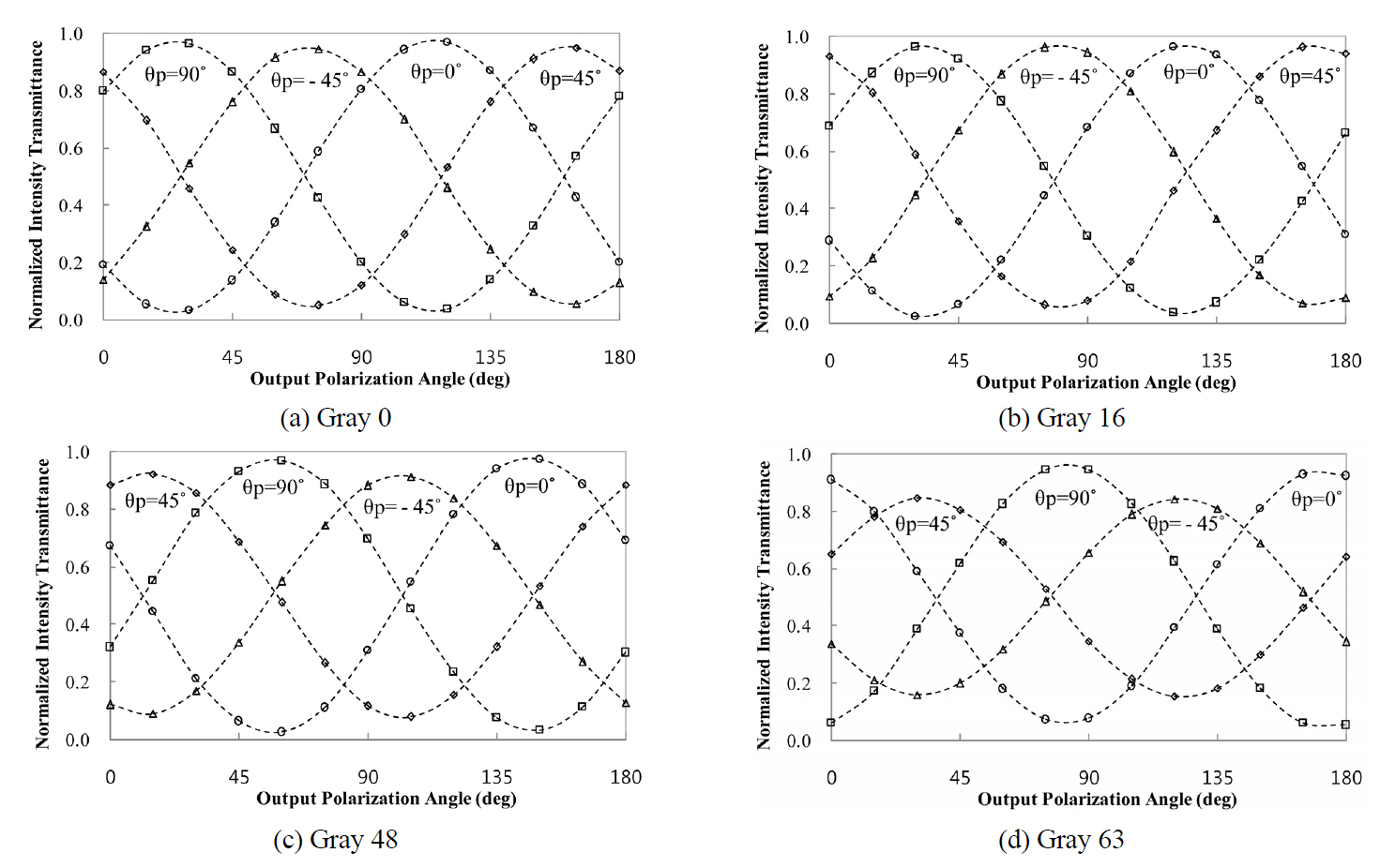
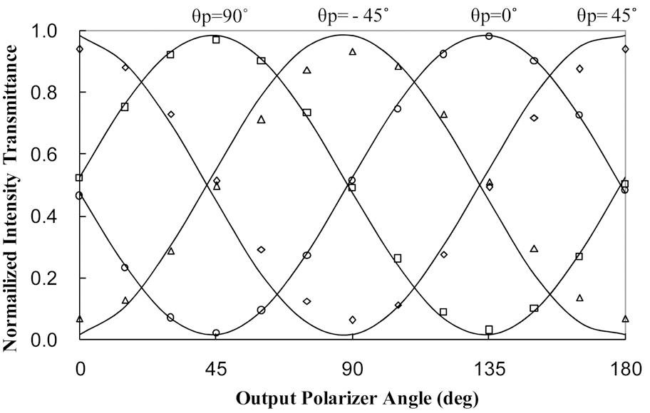
FIG. 2 shows the experimental data of the transmitted intensities for 4 gray levels, 0, 16, 48 and 63. For an
input polarization direction,
Normalized intensity transmittance is measured as a function of output polarization direction.
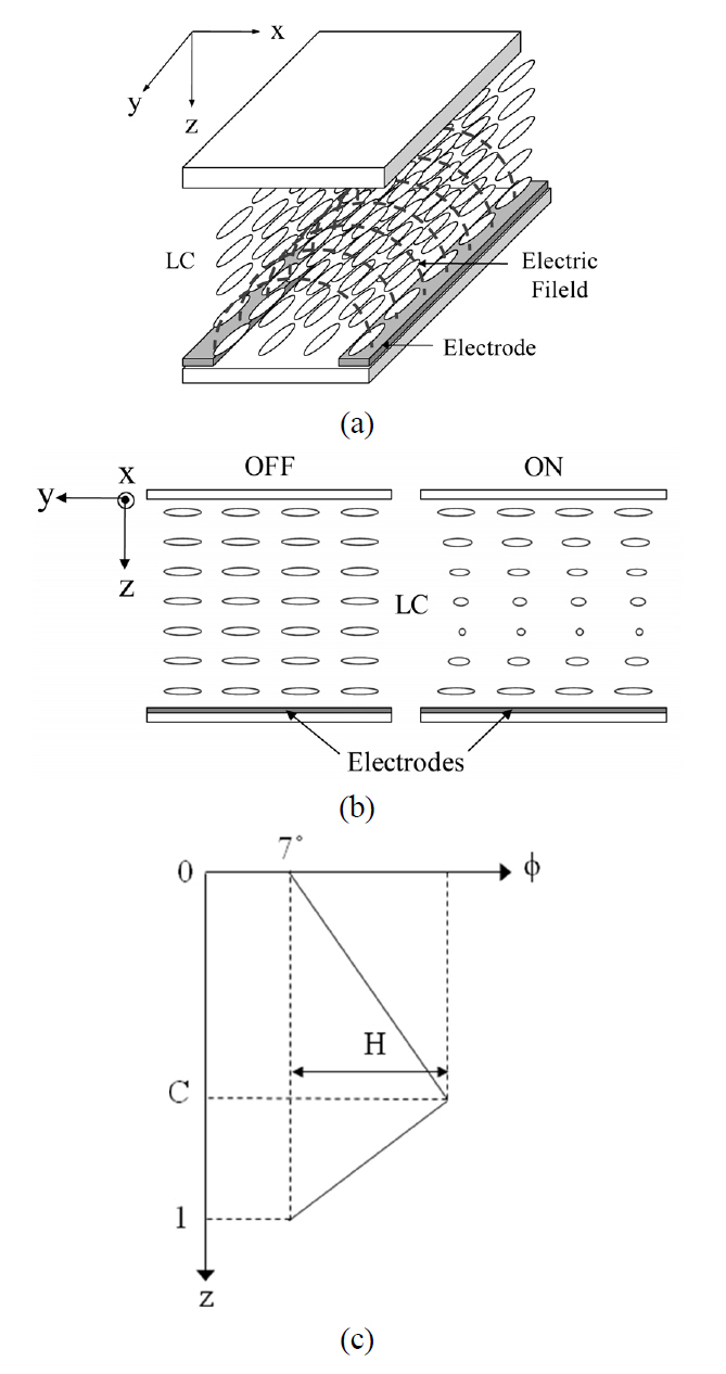
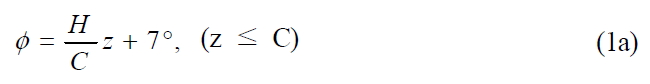
When there is no voltage applied to IPS-LCD, LC molecules are parallel to each other, and align with the rubbing direction of two substrates. The rubbing direction makes an angle of 7 degrees in our IPS-LCD with respect to the+y-axis. FIG. 3(a) is a 3-D perspective of LC molecules with no applied voltage and FIG. 3(b) is its side view.When a voltage is applied to LCD, LC molecules start to rotate toward the +x-axis, whose angle is called the twist
angle. Although the electric field intensity is the maximum at the bottom substrate on which the electrodes are built,the maximum twist of LC molecule occurs near the center region of the LCD, because LC molecules are not free to rotate near the top and bottom substrates. The distribution of LC molecules is so complicated in IPS-LCD that only a 3-D model may predict the exact distribution of LC molecules. However, in this paper, we use a simple 1-D model of IPS-LCD in which it is assumed that the twist angle of LC molecules increases linearly from the top substrate to the center region, and then decreases to the bottom substrate. In this model, the peak twist angle H and the location of the peak C are two parameters that are supposed to be determined from the experimental data.FIG. 3(c) shows our 1-D model of IPS-LCD used in the simulations. An analytic expression for the twist angle of LC molecule is given by
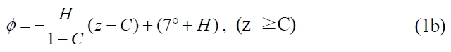
If the system parameters C and H are given, we can calculate the intensity transmitted through LCD by using the standard procedure involving Jones Matrix. In this case, the beam monitored by PD1 gives the input polarization state, while that monitored by PD2 gives the output polarization state. The two polarization states are related by the Jones Matrix equation as
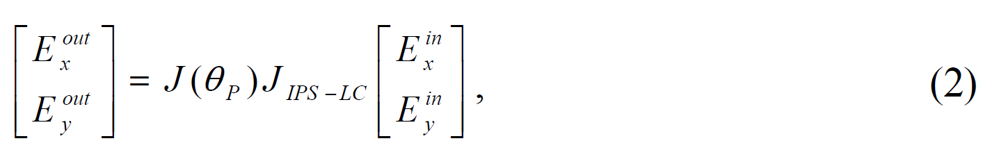
where
where
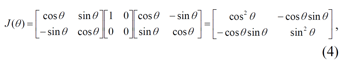
where
The intensity transmittance T is given by the ratio of the measured output intensity
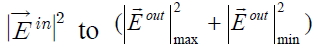

where
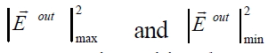
are the maximum and minimum output intensities that are measured by fixing the input beam polarization state. It is customary to write
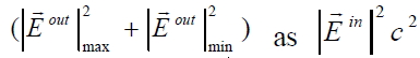
where c is called the loss factor [11, 12]. It is noted that 1-
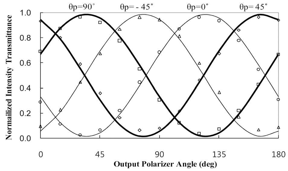
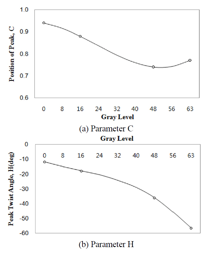
When a gray level is fixed, we obtain the twist angle of LC molecules by fitting Eq. (1) to the experimental data of intensity transmittance. In this case, one might think that more experimental data would result in more accurate values of C and H. However, as we showed in FIG. 2, the intensity transmittance curves repeat themselves every 90 degrees of polarization rotation. In other words, only experimental data with polarization angles in a range of 90 degrees can contribute to the curve fitting. Therefore, we use only two polarization angles for a fixed gray level, which are 45 and 90 degrees. In FIG. 4, the bold lines represent fitting of Eq. (1) to the experimental data of intensity transmittance for the polarization angle of 45 and 90 degrees, when the gray level is fixed to 16. In this case,C and H are calculated to be 0.88 and -17.8 degrees,respectively, as can be seen from FIG. 5. We repeat the curve fitting for gray levels of 0, 16, 48 and 63, and interpolate C and H to obtain smooth curves as shown in FIG. 5. Even if we use intensity transmittances of only two polarization rotations and four gray levels, the interpolations of C and H predict intensity transmittances with very small errors, compared with the experimental data.
In FIG. 5, we know the values of C and H only for gray levels of 0, 16, 48 and 63. For gray level of 32, for example, C and H are obtained from polynomial interpolation given as follows,


where
In the above equations,
To check the validity of our model, we estimate the
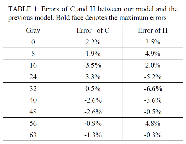
Errors of C and H between our model and theprevious model. Bold face denotes the maximum errors
error in C and H in Table 1. Our model produces C and H as shown in FIG. 5, which are obtained by the experimental data of intensity transmittances for two polarization rotations, 45 and 90 degrees, and four gray levels, 0, 16,48 and 63. We have conducted further experiments to obtain intensity transmittances for 9 polarization rotations(-90, -60, -45, -30, 0, 30, 45, 60, and 90 degrees), and 9 gray levels(0, 8, 16, 24, 32, 40, 48, 56, and 63). We have repeated curve fittings to these experimental data to obtain,so called, “C and H of all data”. Table 1 shows percent errors between C and H of our model and those of all data. We note that the maximum error of C is estimated to be 3.5% and the maximum error of H to be 6.6%. It shows that our model produced little error.
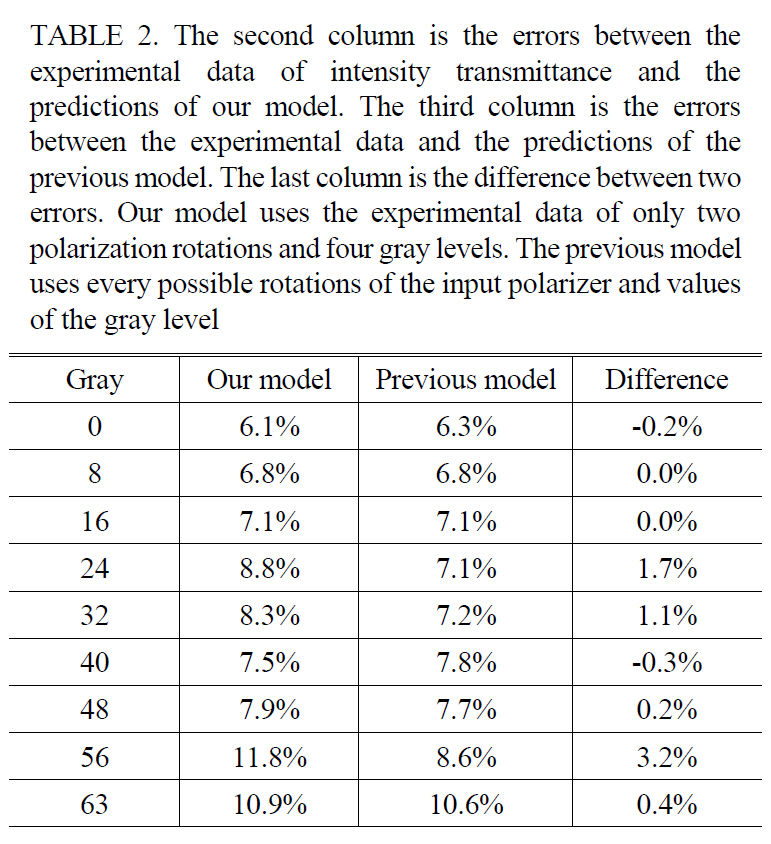
Next, we compare the intensity transmittances of our model and the experimental data. The second column of Table 2 shows percent errors between intensity transmittances predicted by our model and those measured in the experiment.The third column shows percent errors between intensity transmittances predicted with C and H that are obtained from all data, and the experimental data. The fourth column

The second column is the errors between theexperimental data of intensity transmittance and thepredictions of our model. The third column is the errorsbetween the experimental data and the predictions of theprevious model. The last column is the difference between twoerrors. Our model uses the experimental data of only twopolarization rotations and four gray levels. The previous modeluses every possible rotations of the input polarizer and valuesof the gray level

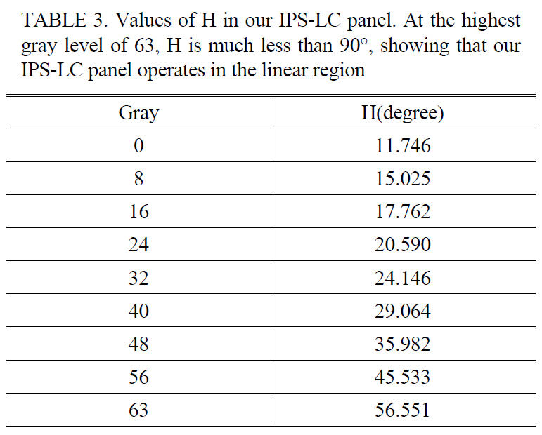
Values of H in our IPS-LC panel. At the highestgray level of 63, H is much less than 90°, showing that ourIPS-LC panel operates in the linear region
is the difference between the two percent errors. The comparison shows that our model agrees excellently with the experimental data, with the maximum error less than 12%.When all data are used, the error is reduced only by 3.2%.The values of H in Table 3 show that our IPS-LC panel operates in the linear region.
We have measured the intensity transmittance through an IPS-LC panel by changing the gray levels, and by changing the directions of the input polarizer and the output polarizer. From the experimental data we have observed that the intensity transmittance curve repeats itself, in its shape, every 90 degree of the polarization direction. Next,by fitting the one-dimensional model to the experimental data, we have measured the parameters C and H as functions of gray levels. The curve fitting shows that the C and H curves are more sensitive to the values at the gray levels near zero and near the maximum 63. Based on these new observations, we reform the one dimensional model such that it uses only the experimental data of polarization rotations of 45 and 90 degrees, and the experimental data of four gray levels of 0, 16, 48, and 63. The previous model uses every possible rotation of the input polarizer and every possible value of the gray levels on the premise that more data would produce more accurate fitted parameters of LC panel.[10] When the predictions of our model, for C and H, are compared with those of previous model, the error is estimated to be less than 3.5%and 6.6% for C and H, respectively. The predictions of our model are also compared with the experimental data of intensity transmittance. In that case, the error is estimated to be less than 11.8%. Since the previous model produces the maximum error of 10.6%, we can conclude that the errors of 11.8% and 10.6% just result from the limit of the one dimensional model. Although our model uses a limited amount of experimental data in determining the parameters C and H, the predictions for the parameters and the intensity transmittance are excellent when they are compared with the experimental data.