Visual navigation, robotics and vision-based measurement are just a few examples of industrial applications that depend on pose estimation and computation of the three-dimensional(3D) object location[1-7]. In 3D reconstruction process with an optical technique, system accuracy is defined as a problem of the determination of 3D point positions, which are provided by 2D features gathered from binocular calibrated cameras. For great accuracy in the system performance, camera calibration and reconstruction have to be accurately performed.
In the past many researchers have developed algorithms for camera calibration and reconstruction as an open topic in computer vision. Currently, several major calibration techniques are available. The most popular camera calibration method is the direct linear transformation (DLT) method originally reported by Abdel-Aziz and Karara[8]. The DLT method uses a set of control points whose object space coordinates are already known. The control points are normally fixed to a rigid calibration frame. The flexibility of the DLTbased calibration often depends on how easy it is to handle the calibration frame. The main DLT method problem is that the calibration parameters are not mutually independent. An alternative approach is reported by Hatze to ensure the orthogonality of the rotation matrix[9]. The direct nonlinear minimization technique directly builds camera parameters to minimize the residual error utilizing iteration computation[10, 11]. The intermediate parameters can be computed by solving linear equations. However, lens distortions do not follow this method[12, 13]. Len[14] and Tsai[15, 16]introduce an improved solution for calibration which is a two-step method to compute the distortion and skew parameters.To make the calibration more convenient and to avoid requiring 3D coordinates, Svoboda[17] made the technique more robust. According to the analysis of several images of a 2D calibration board, usually with a chessboard pattern, Z. Zhang[18, 19] describes an efficient method to improve the accuracy of the camera calibration based on Tsai’s model. A similar technique is explained by Kato[20], who focuses on retrieving camera location using fiducially markers, which are located in the 3D environment as squares of known size with high contrast patterns in the centre. K. C. Kwon[21] proposes a binocular stereoscopic camera vergence control method using disparity information by image processing and estimates the quantity of vergence control.
For evaluating the calibration accuracy, K. Zhang[22] explores a model of the binocular vision system focused on 3D reconstruction and describes an improved genetic algorithm aimed at estimating camera system parameters.In order to enhance the calibration accuracy, many corners should be treated as feature points, which are distributed uniformly on the calibration block. W. Sun[23] presents a study investigating the effects of training data quantity, pixel coordinate noise on camera calibration accuracy. H. H.Cui[24] discusses an improved method for accurate calibration of a measurement system. The system accuracy is improved considering the nonlinear measurement error. Independent of the computed lens distortion model or the number of camera parameters, C. Ricolfe-Viala[25] outlines a metric calibration technique that calculates the camera lens distortion isolated from the camera calibration process. An accurate phase-height mapping algorithm is proposed by Z. W. Li[26] to improve the performance of the structured light system with digital fringe projection. By means of a training network, the relationship between the 2D image coordinates and the 3D object coordinates can be achieved. However, their experiments involve fixed system structure parameters and provide neither a synthetic evaluation on separate test data nor flexible binocular system parameters to verify the accuracy calibrated results.
Considering the widely used DLT calibration method, we emphasize the structure factors that influence the binocular measurement system accuracy in this paper. Baseline distance and measurement distance are evaluated and applied to the experimental binocular system to reveal the quality of each factor. In the experiment, the 3D board calibration method for both factors is applied.
The calibration method requires a set of 3D coordinates and two sets of 2D coordinates of grid board images from two cameras. Then the intrinsic and extrinsic parameters are calculated by solving the projection equation.
where
where
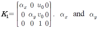
are the focal lengths along
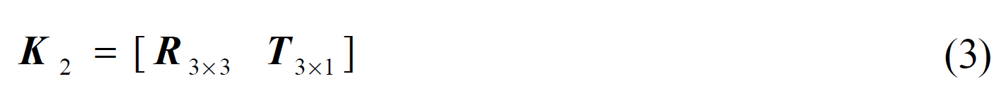
where
3D reconstruction is usually applied in the binocular vision measurement where the camera projection matrices of two cameras are adopted to calculate the 3D world coordinates of a point viewed by the cameras. Suppose
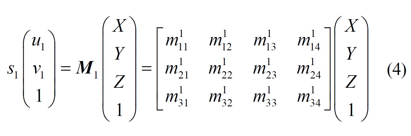
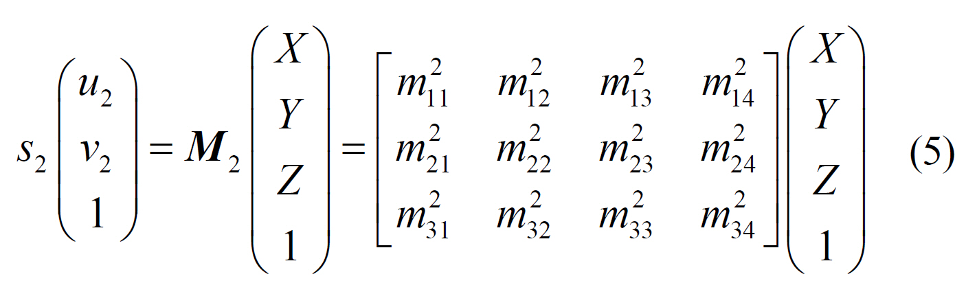
where (
Derived from Eq. (4) and (5), two scalars
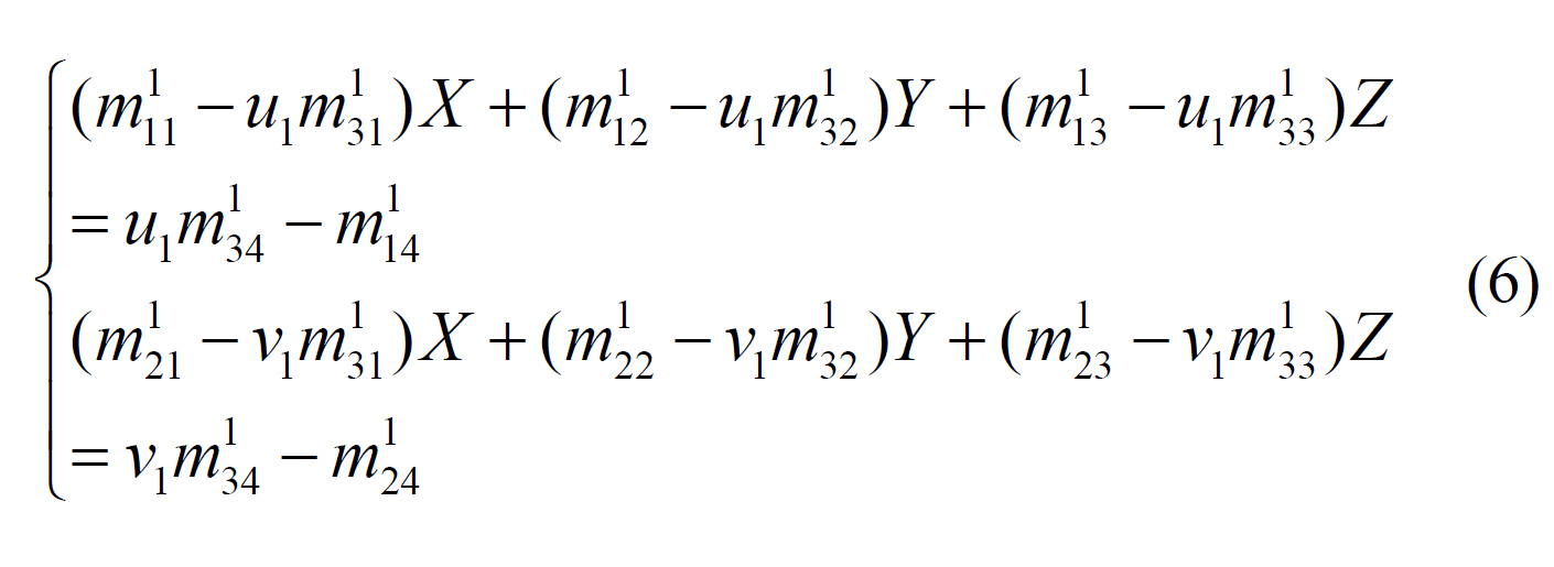
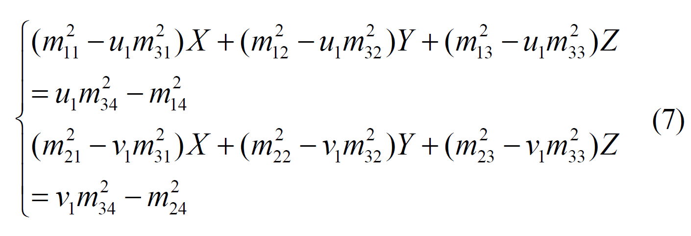
Since one linear equation stands for a plane in space and two composite linear equations represent one crossing line of two planes, Eq. (6) and (7) refer to two lines in 3D space, which intersect at the 3D point
III. EXPERIMENTAL METHODS AND RESULTS
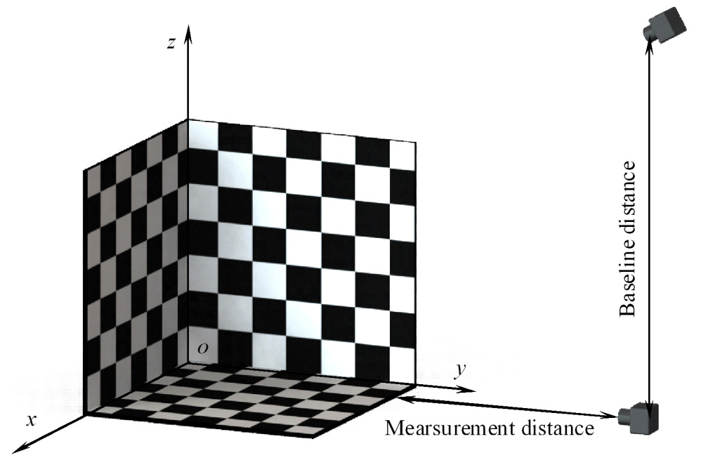
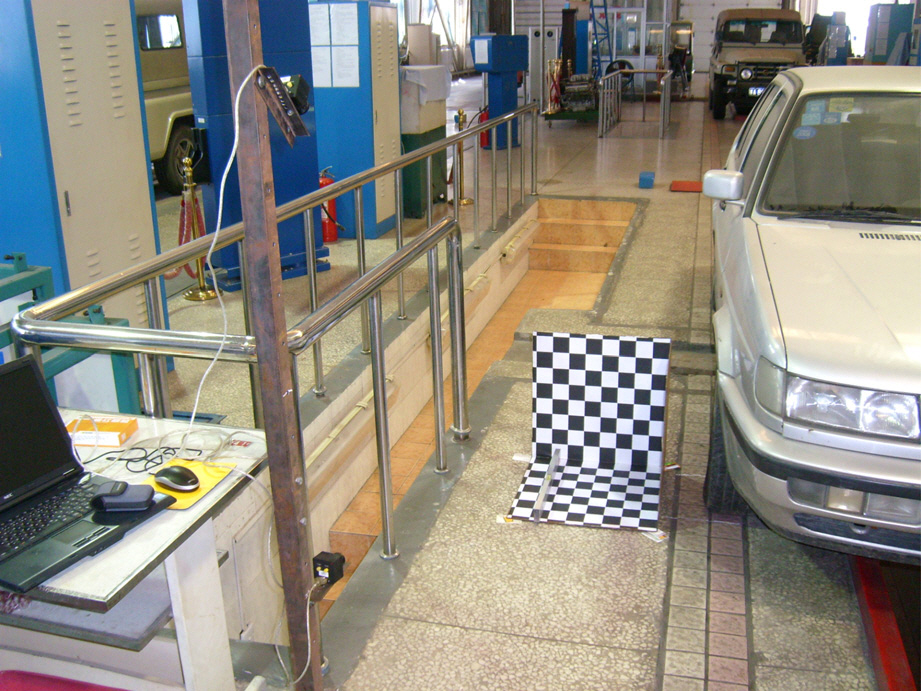
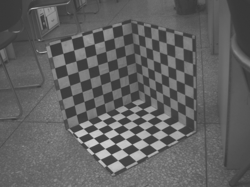
The experiment is carried out in our laboratory space equipped with a vertical rack, raised about 2 m above the ground, as shown in Fig. 1. Two DH-HW3102UC cameras with 8 mm focal length lens are placed along the rack in a line perpendicular to the horizontal plane. The image resolution is 2048×1536 pixels with the frame rate 6 frame/sec and pixel size 3.2 ㎛×3.2 ㎛. To investigate the influences of baseline distance and measurement distance illustrated in Fig. 2., twenty-five configurations, baseline distances of 600 mm, 800 mm, 1000 mm, 1200 mm, 1400 mm, and measurement distances of 1000 mm, 1500 mm,2000 mm, 2500 mm, 3000 mm, are separately studied on the experimental setup.
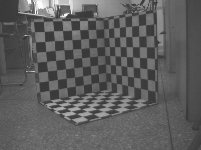
The obtained data for calibration is generated by printing a chessboard pattern of 60×60 mm grid corners onto three 500×500 mm sized sheets. Each of them is attached to the plane of a rigid cube. Binocular images captured from two cameras are demonstrated in Fig. 3. and Fig. 4. It produces two 2D coordinate data sets of 27 points for either camera.
The 3D world coordinates of these points are measured relative to the intersection point of three chessboard pattern sheets, i.e. the origin of world reference system. The 3D coordinate data set has covered the calibration cube surface with 60 mm division. Because a normal ruler is accurate only to 1 mm, the maximum calibration board error of 0.5 mm can be reached, which is approximate 0.83% of the pattern size.
3.2. Accuracy Evaluation Results
The calibration result is a set of camera parameters. In most applications, the parameters are used for stereo computation to reconstruct the 3D coordinates for feature points of the measured objects. As the baseline distance, the measurement distance and the measurement direction are the three essential factors for the feature point reconstruction precision, the influences should be evaluated by the accuracy experiments of the stereo vision system.
In this evaluation, with given camera parameters, stereo computation reconstructs the 3D coordinates of feature points on the calibration board by 2D camera images. Since the measurement and baseline distances of a binocular system influence the system accuracy, the difference between the reconstructed 3D coordinate of a feature point and the original coordinate in space is defined as the stereo error. The stereo error is related to the camera parameters and is restricted by system structures. To make a conclusion, we create a binocular system and choose some synthetic test points to show the stereo error distribution in 3D space. Furthermore, since different test points have different error values, we also analyze the error distribution and scope to show the relationship between the stereo error and the positioning parameters of the binocular system. The identical calibration and reconstruction methods mentioned above are adopted to ensure that the assessment results are independent of the computation method. Therefore, different measurement results are appraised with the same evaluation procedure.
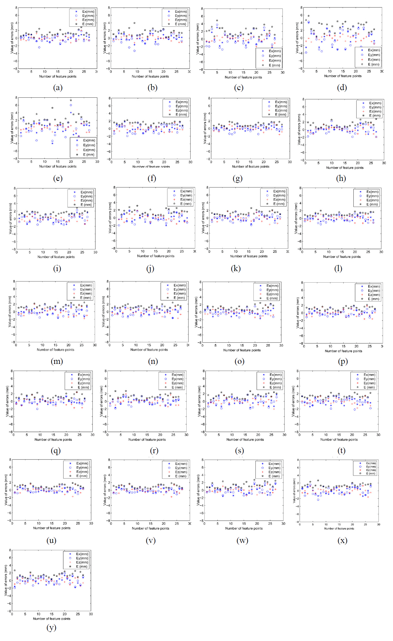
The stereo error varies when the camera positions are different. The 3D errors are defined as follows:
where (
Fig. 5(a)-(y) attempt to show what level of accuracy is available given a constant amount of baseline distance and a variable observation distance. All the data are collected under similar conditions in order to compare experimental results.
In the scope of the error distribution in Fig. 5(a)-(y), as the measurement distance increases from 1000 mm to 3000 mm, the maximum error value changes from -2 mm - +2 mm to -4 mm - +6 mm, and the error values distribute more dispersedly. From these results, we come to the conclusion that the error value increases with the distance between the test object and the measurement system. However, when the baseline distance varies from 800 mm to 1400 mm with a certain constant value of measurement distance 1000 mm,1500 mm, 2000 mm, 2500 mm, or 3000 mm, for example, 3000 mm, the error value transforms from -4 mm - +6 mm to less than -2 mm - +2 mm in the boundary of error scope. If the baseline distance is increased, the measurement system error made by binocular cameras is reduced. Since the baseline distance is confined with system dimensions and the error distribution concentrates on -2 mm to +2 mm when the baseline distance is up to 1000 mm, the optimal value of the system is baseline distance 1000 mm, measurement distance 1500 mm with the minimum error value and distribution scope. For a certain binocular measurement system, after an obvious peak of the accuracy benefit from baseline distance increase, the system accuracy is not able to be improved effectively. In addition, we notice that the measurement error in the
3.3. Experimental Results Discussion
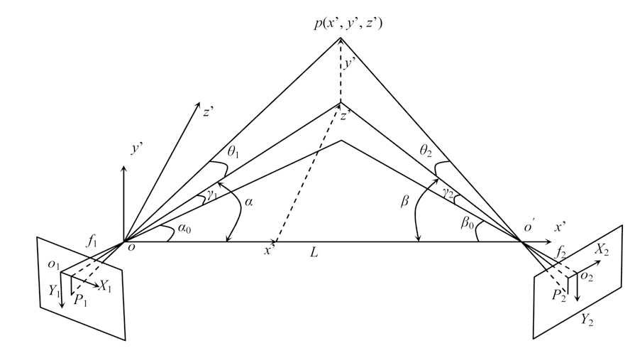
A model of the binocular measurement system is constructed in Fig. 6, where
For evaluating the measurement error caused by baseline distance variation, the error transfer function relative to baseline distance,
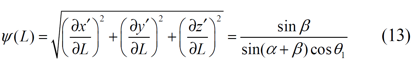
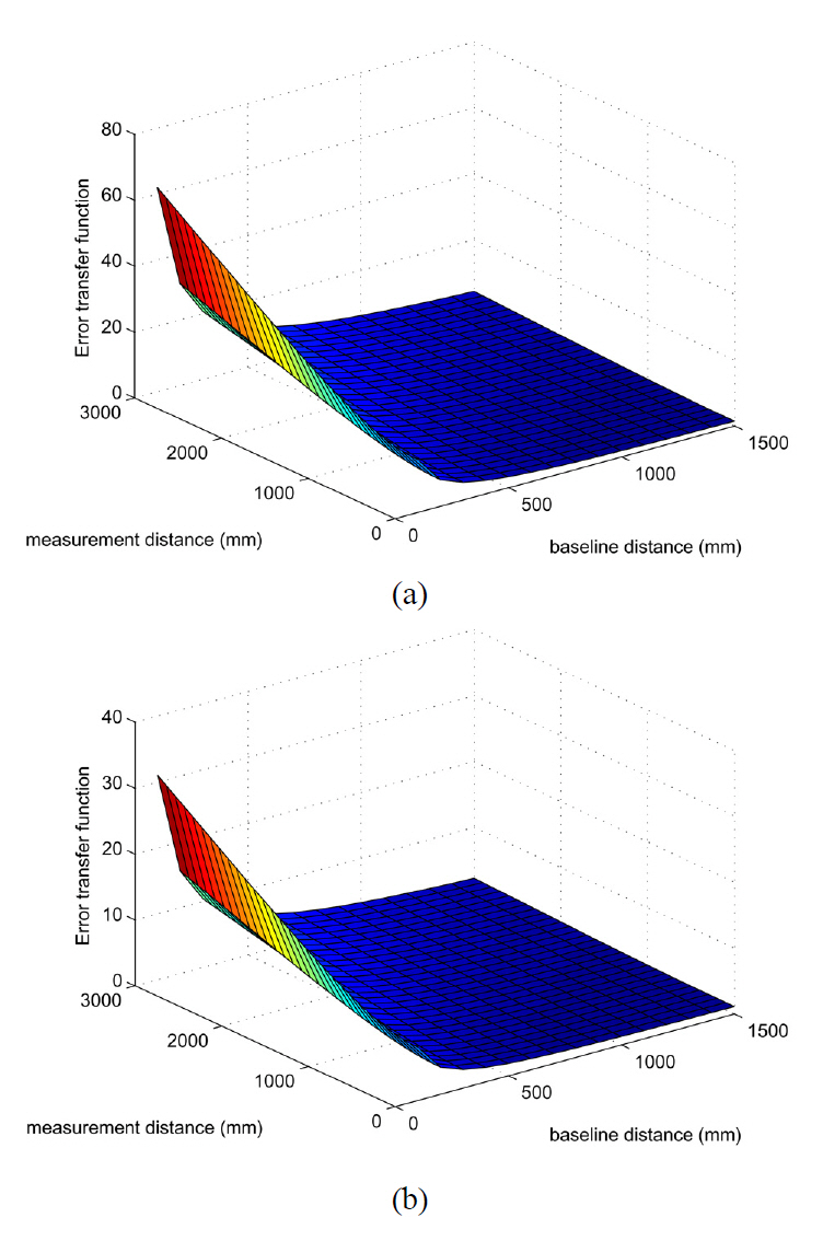
Here, two typical situations are considered in this paper,
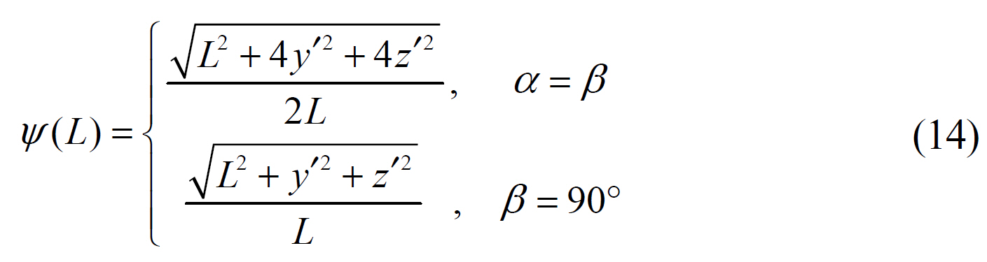
Where
According to simulation results in Fig. 7, the value of error transfer function reduces as the baseline distance
An experimental study on camera calibration and 3D reconstruction of a binocular measurement system is carried out to investigate how factors such as baseline distance, measurement distance and baseline direction affect the reconstruction accuracy. The most representative method, developed by Abdel-Aziz and Karara, is chosen for experimentation on 2D data from cameras. A typical criterion is applied to evaluate measurement accuracy on test sets.
With the same reference calibration board, we set a series of test distances from 1000 mm to 3000 mm based on the same calibration and reconstruction methods. According to the comprehensive error, a smaller test distance employing grid-board calibration shows a more stable result than a higher distance method. Nevertheless, the value of the measurement distance of a binocular system is determined on the detected object, system geometrical structure and view field. Therefore, it is an inefficient method to enhance accuracy by adjusting measurement distance between cameras and the detected object in the experimental situation that the measurement distance is constrained by the system structure and camera characteristics. If we alter the baseline distance for the source data of the binocular system, the accuracy is more sensitive in the range of 600 mm to 1000 mm. Thus, to increase the accuracy of the binocular system, it is more important to increase the baseline distance than to improve the measurement distance. However, experimental results indicate that after a peak of accuracy, i.e. 1000 mm in the experiment, it is unproductive to improve measurement effects by choosing a larger baseline distance.
The stereo error evaluation shows that the measurement result gotten in different directions has different valid ranges. For the
In summary, it is clear that the methods for enhancing accuracy of a binocular measurement system depend greatly on some known specific geometrical information such as the test object dimension, measurement distance, baseline distance and direction. Hence, it is crucial to select a reasonable system dimension and structure for binocular measurement so as to improve the accuracy of 3D feature measurement precision using binocular vision.