In the beginning of the 20th century, water quality problems were largely related to issues of waterborne disease and oxygen demanding organic material. As higher levels of nutrients were introduced to surface waters due to increased uses of fertilizer or phosphate containing detergents, eutrophication became one of the major water quality issues. In recent years, toxic material including synthetic organic chemicals and heavy metals have gained increased attention due to their potentially harmful effects to human health.
As demand for better water quality has increased, water quality models have become important tools in water quality management related decision making processes. As accurate quantification of required load reductions is the most important factor in the implementation of legal frameworks such as the Total Maximum Daily Load (TMDL) program in the United States and the Total Waste Load Management Act in Korea, the role of water quality models has become more important.
Since the pioneering work of Streeter and Phelps [1] in the mathematical modeling of the DO-CBOD relationship, water quality modeling has been expanded and improved [2]. The USEPA has made significant contributions in the field of water quality modeling by developing, managing and upgrading publicly available water quality models such as QUAL2E [3], WASP[4], SWMM [5], and HSPF [6].
The QUAL2E model is one of the most widely used models in recent decades. BASINS3.1 [7], the integrated water quality modeling interface to support TMDL development in the United States, uses QUAL2E as the only stream water quality model in the program. Korea launched the Total Waste Load Management Act in 2003 to protect its major river water quality [8],and has used the QUAL2E model to develop water quality standards at major points along its river systems. Wide application of QUAL2E, however, does not necessarily mean that the model is without limitations. As an alternative, Park and Lee [9] suggested a modified version of the QUAL2E model by adding the effect of dead algae on carbonaceous biological oxygen demand(CBOD) and nitrogen loss due to denitrification. Chapra et al.[10] developed the QUAL2K stream water quality model that has a larger number of constituents with more detailed water quality processes that can consider dynamic water quality kinetics given steady flow conditions. Ambrose et al. [11] gave an excellent summary on historical trends in water quality model development in the United States.
Though many advanced modeling techniques are available,steady state modeling approaches are still widely used, especially for governmental decision making processes. In this regard,the following issues need to be considered.
Firstly, although QUAL2E and other similar models are capable of modeling detailed nutrient cycle processes, water quality standards are often developed for ”total” concentrations such as CBOD, the total nitrogen (TN), or the total phosphorus (TP).Thus, if only total pollutant concentrations are needed, then it should be simpler and equivalently accurate to model the total constituents directly rather than modeling detailed processes for individual components and add them later. This outcome results primarily from the difficulty in reliably estimating so many reaction rates for individual components. When modeling total pollutant levels only, the benefit of detailed information for model inputs can be minimal and the modeler may avoid the greater uncertainty due to propagated errors from many uncertain inputs.
Secondly, the QUAL2E model and other similar models use Manning’s method or a rating curve method to calculate steady water velocity and depth. Both methods require the principle of continuity. However, often small streams may not satisfy this theoretical requirement since water flow may become discontinuous along the stream. Continuity may be satisfied for small streams when the watershed area is dominated by impervious surfaces or streams with extremely low base flows.
The velocity of water directly affects hydraulic retention time and exit concentration of a pollutant from a control volume of interest. Therefore, improper assessment of hydraulic retention time may cause serious problems in the calibration of the model and thus mislead the interpretation of the water quality kinetics of the study area.
In this paper, the authors emphasize that the level of model complexity needs to be compatible with the modeling objectives,and the structure of the model is preferred to be as simple as possible. The suggested CAP model will do this job for many current water quality management related decision making processes.
The general mass balance relationship for any water quality constituent in a volume of water can be expressed as the sum of the derivatives for advection, dispersion, reaction, sources, and sinks:
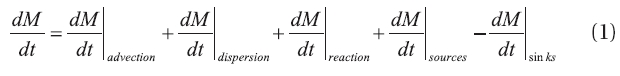
where, M is the mass of a constituent (mg).
The mass derivatives due to advection and dispersion are caused by physical transportation processes in the water system.These are often calculated by using hydraulic or fluid mechanics principles. Sinks are usually caused by physical removal of water,such as withdrawals via intake facilities. For a homogeneous water volume, advection, dispersion, and withdrawal affect every water quality constituent in the same manner (except for immiscible fluids, which are not considered here). On the other hand, reactions and sources are material-specific and need to be considered for each individual constituent separately.
For natural streams, advection is generally the dominant factor in mass transfer. The presence of an in-stream structure,however, can significantly lengthen hydraulic residence time in a river reach so that dispersion or reaction processes can become dominant factors in the absence of additional sinks or sources.Depending on the situation, in-stream structures may cause intermittent or discontinuous flow especially for streams that have minimum inflow from the watershed or have low base flow conditions. Most water quality models that include a hydraulics module, such as QUAL2E, require a mass balance relationship or continuity in the flow for the entire system. Therefore, if flow in a stream is discontinuous, it becomes inappropriate to apply those models.
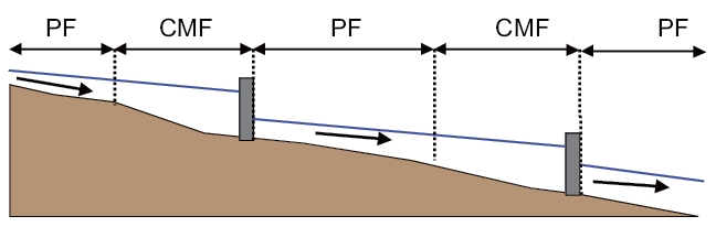
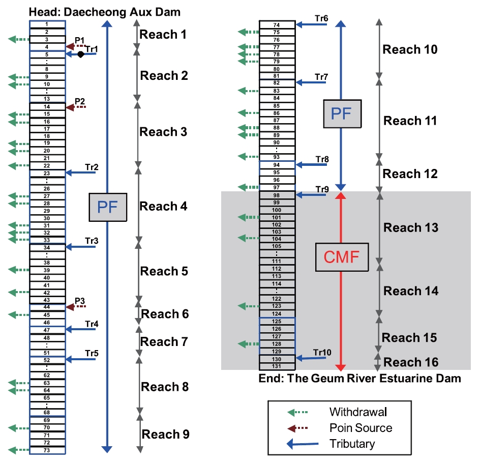
Seo and Lee [12] developed a CAP (CMF And PF) water quality model to overcome this problem. Free flowing reaches of a stream can be treated as plug flow (PF) reactors. Stagnant flow reaches formed by in-stream structures can be treated as completely mixed flow (CMF) reactors. As shown in Fig. 1,a CAP model considers a stream as a combination of PF reaches and CMF reaches. At the outlet of each CMF reach, where flow may be discontinuous due to hydraulic structures, users can reset the headwater condition.
2.2. Hydraulic Characteristics
For free flowing plug flow reaches, it is necessary to provide adequate hydraulic information to appropriately represent advection. For these reaches, the CAP model assumes a steady state hydraulic regime as in the QUAL2E model [3] or the QUAL2K model [10]. In the most commonly used rating curve method, hydraulic information for a reach can be estimated by using the following equations:
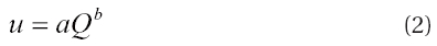
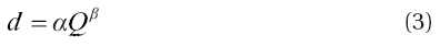
where, u and d are the average segment velocity (m/sec) and the average segment depth (m), respectively, and a, b, α, β are empirical constants.
2.3.1. CBOD
CBOD is an index of the consumption potential of dissolved oxygen in the water. Oxygen depletion can be caused by chemical reactions and by algal and bacterial respiration. The reaction rate of CBOD is often expressed as a first order reaction as follows:
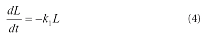
where, L is the ultimate CBOD concentration (O2 mg/L); k1 is the deoxygenation coefficient (1/day).
For settleable oxygen requiring organic material, Equation(4) can be modified to represent a first-order settling rate as follows:
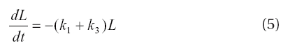
where, k3 is the settling rate of CBOD (1/day).
The above relationship was used in the QUAL2E model. However,QUAL2E ignores the effect of algal death [4] and denitrification[9] on CBOD concentration in the system. If these effects are included, the CBOD reaction equation can be modified as follows:
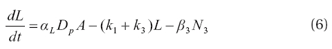
where αL is the fraction of algal biomass that is converted to CBOD following death (mg-CBOD/mg-A), A is the algal concentration(mg-A/L) , N3 is the nitrate concentration (mg-N/L), Dp is the algal death rate (1/day), and β3 is the nitrate nitrogen denitrification rate (1/day).Chapra [
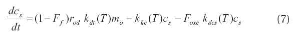
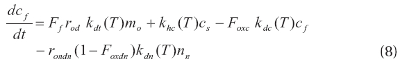
chapra [10] partitioned CBOD into slowly reacting (CBODs)and fast reacting (CBODf). It is assumed that CBODs and CBODf are gained by detritus dissolution. CBODs is lost via hydrolysis and oxidation, and CBODf is lost via oxidation and denitrification.It is also assumed that hydrolyzed CBODs is a source of CBODf. These two different CBOD components represent dissolved CBOD in the water, and their reaction rates can be expressed as:
where
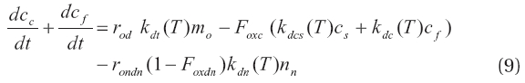
If the effect of particulate material is included, the total CBOD reaction rate can be expressed as follows:
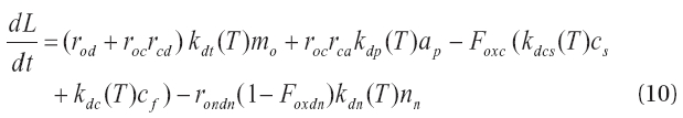
where, roc, rca, and rcd are the ratio of oxygen equivalents lost per carbon, the ratio of carbon equivalents lost per algae, and the ratio of carbon equivalents lost per detritus, respectively; ap and mo are the algae or chlorophyll A concentration particulate organic matter concentration, respectively;
Low oxygen levels are required for the denitrification process to occur. Therefore, denitrification can be ignored in most shallow streams where sufficient oxygen concentrations are maintained.If a stream has turbulent flow that can inhibit the growth of algae, the effect of algae and organic material in Equation (10)also can be ignored. If CBOD exists entirely in soluble forms in the water, then Equation (10) can be reduced to a first order reaction process as follows:
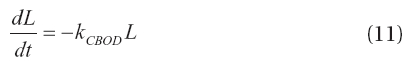
where, kCBOD is first order reaction coefficient of CBOD (1/day).
2.3.2. TN and TP
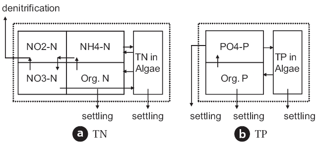
Kinetic reaction processes can cause a segment to lose or gain mass depending on the reaction characteristics of a constituent.QUAL2E [3] divides the total nitrogen into organic, ammonia,nitrite and nitrate nitrogen, and the total phosphorus into organic and dissolved inorganic phosphorus. The WASP model[4] uses nitrate as a combined variable for nitrate and nitrite. The QUAL2K model [10] and the WASP7 advanced eutrophication module [13] calculate the free ammonia (NH3) concentration,which becomes significant under high pH conditions.
Though there may be several different speciation methods for the composition of the total nitrogen or the total phosphorus,their overall reaction can be summarized as in Fig. .2 If a system is aerobic where denitrification will not occur, the kinetic loss of both the total nitrogen and the total phosphorus will be governed only by settling processes. Therefore, it should be rea-
sonable to express these kinetic process relationships as first order reactions for an aerobic surface water system:
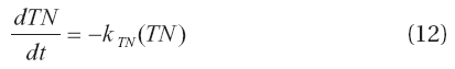
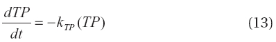
where, kTN and kTP are the first order reaction coefficient of TN(1/day) and the first order reaction coefficient of TP (1/day), respectively.
The mass balance equation for a constituent that follows first order reaction kinetics in a one-dimensional reach can be expressed as follows:
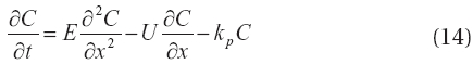
where, C is the concentration of water quality constituents of interest (mg/L), E is the dispersion coefficient (m2/day), U is the water velocity in the x-direction (m/day), and kp is the first order reaction coefficient (1/day).
UL/E is defined as a Peclet number (Pe) that represents the ratio between the rate of advective transport and the rate of diffusive/dispersive transport [14]. If Pe is greater than 10, it is assumed that the one-dimensional reach can be treated as an idealized plug flow reactor with no longitudinal mixing [14, 15].Neglecting dispersion, the steady-state solution to Equation (14)is:
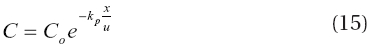
where, Co is the concentration of a constituent entering the head of the reach.
If the dispersion coefficient is very large, or Pe is less than 10,then the entire reach can be treated as a completely mixed reactor.The mass balance equation and steady state solution would then be written as follows:
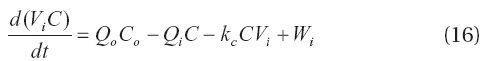
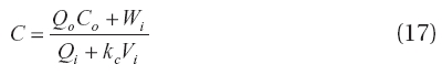
where, kc is the first order reaction coefficient (1/day), Q is the inflow rate or outflow rate for the ith CMF section (m3/day), Vi is the volume of a CMF section (m3), and Wi is the pollutant loading to the ith CMF section (mg/day), respectively.
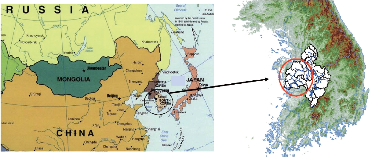
2.5. Study Site: The Geum River, Korea
The Geum River is the third largest river in Korea; it is 401 km long with a basin area of 9,313 km2. The location of the river is shown in Fig. .3The study site is located in the downstream section of the Geum River, stretching 132 km from the Daecheong Auxiliary Dam to the Geum River Estuarine Dam near the coast.Due to increased development in the basin, the level of pollutant loading and water quality concentrations in the river have increased. Since several local governments share boundaries in the river, there have been concerns over sharing of responsibilities for water quality management of the river.
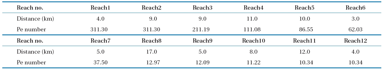
Fig. 4 shows the model network, along with point sources and withdrawals. It was assumed that the agricultural withdrawal occurred only during the active farming period between April and September. All the tributaries were treated as point sources in this study using observed data. When flow data was not available,monthly flow rates were estimated by considering the flow per basin area. If there was any known artificial input, the data was included in the flow calculations. Intensive water quality and flow data was collected along the 132 km study area between March 2002 and December 2003 for calibration and verification of the model. The study site was divided into 16 reaches for the CAP model application. The upper 12 PF reaches were assumed as PF reaches and the rest of the downstream reaches were treated as a CMF reach, based on Peclet numbers measured in the low flow period, as shown in Table 1.
In order to compare CAP model results with a traditional modeling approach, QUAL2E was applied to the study site using the same input for reaches 1 through 12. Reaches 13 through 16 were treated as plug flow in QUAL2E, and as a single CMF reach in CAP (Fig.4 ). To better estimate the hydraulic constants required by QUAL2E and CAP, HEC-RAS [16] was applied under various flow conditions. From March through June, the water level in the Geum River Estuarine Dam is maintained at >2 m.For the rest of the year, the water level is maintained at >1 m.Hydraulic constants were estimated for the two different periods and applied to the CAP and QUAL2E models equally in this study.
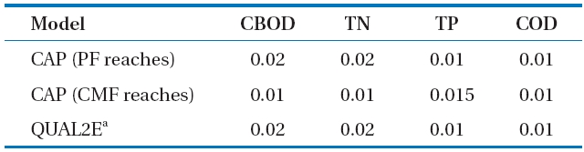
The CAP and QUAL2E models were calibrated using data collected in September of 2002. Reaction coefficients were adjusted by trial and error until predicted CBOD, TN, and TP concentrations fit the observed data throughout the study area. Special attention was paid to verify the model using data collected in November and December of 2002. Table 2 shows calibrated parameters at 20oC for each model. In the QUAL2E user’s manual,the USEPA suggests that the BOD decay rate and settling rates can vary between 0-10/day. Bowie et al. [17] showed that deoxygenation rates were determined for rivers and estuaries in the range of 0.004- 4.25/day from field and laboratory studies.In general, the decay rates in natural waters tend to be smaller than for laboratory-derived rates due to resuspension or generation of organic material in natural rivers. As shown in Table 1,the
authors found the decay rate in the range of 0?0.02/day can be effectively used under the given conditions. Adams [18] summarized literature values for the organic matter settling velocity. According to her table, the typical settling velocity of organic material ranges between 0.01?2.3 m/day. If the average depth of the study area is assumed to be 3 meters, the first order loss rate of TN and TP can range between 0.003?0.8/day. The calibrated parameters seem to be in the lower bound of the literature values.However, by considering the loss rates as lumped parameters that may include possible release or re-suspension, the calibrated values seem to be reasonable. Temperature correction factors of 1.047 for BOD decay and 1.024 for organic settling [3] were applied, respectively, for both models when the parameters were used for different months.
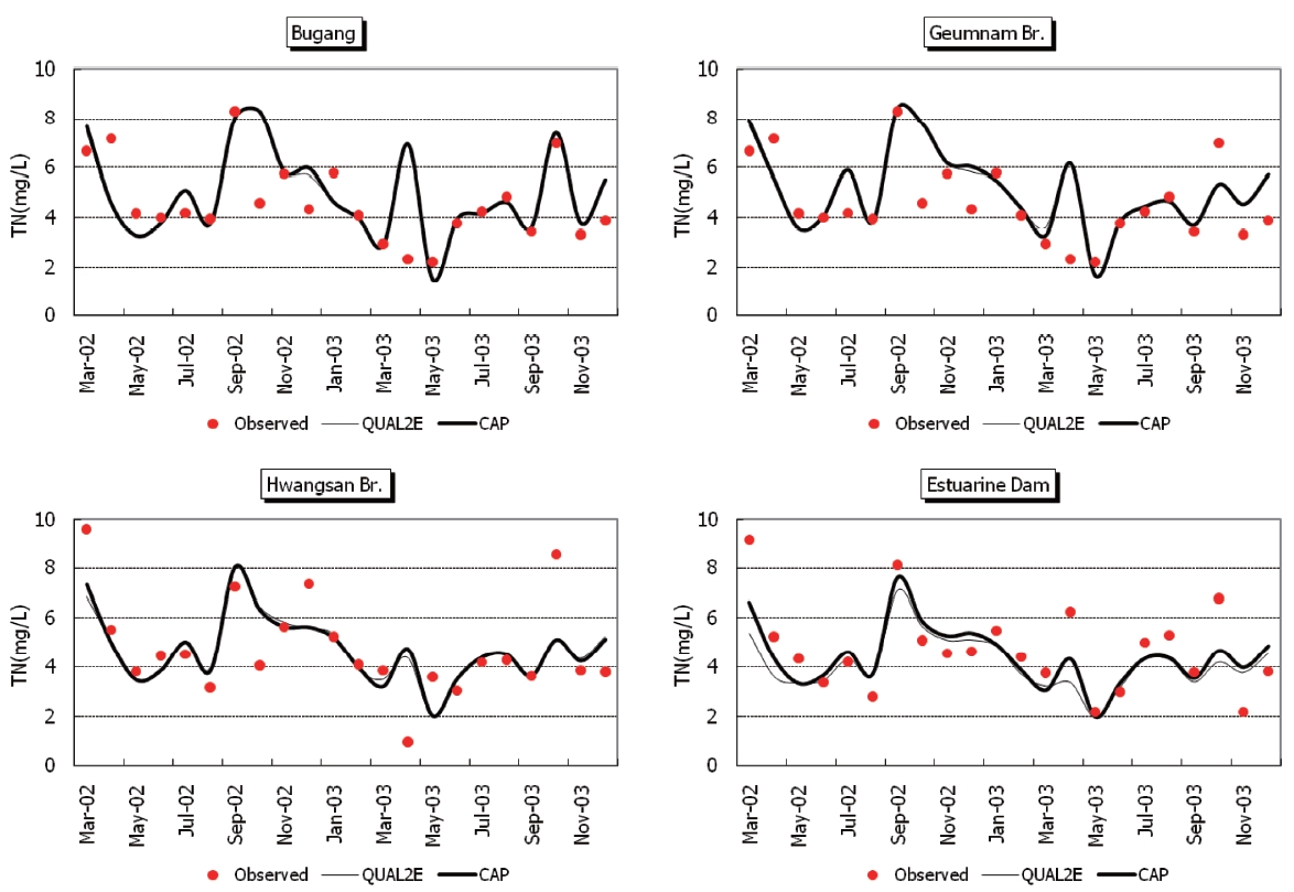
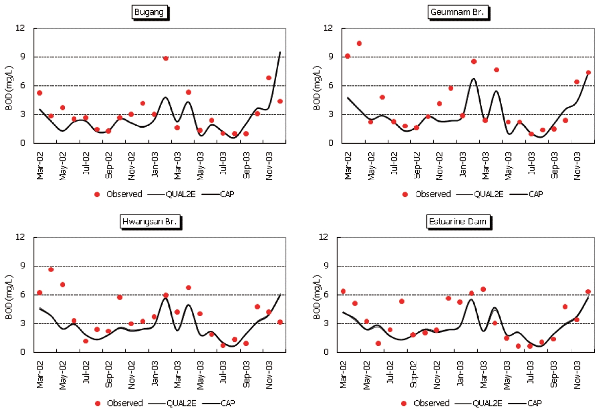
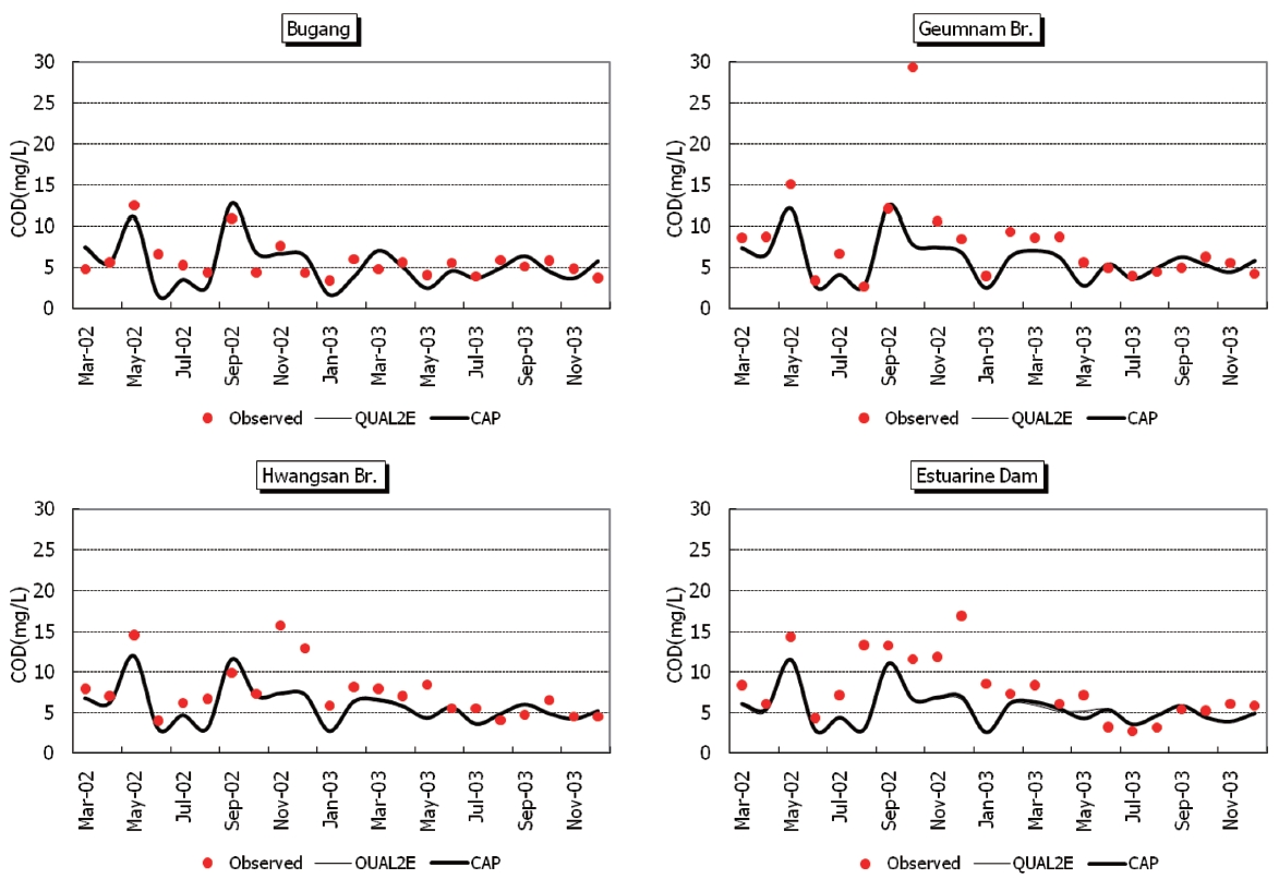
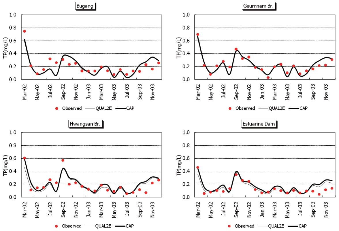
Observed and predicted concentrations of CBOD5, COD, TN,and TP at four stations are shown in Fig. 5 through Fig. .8 As displayed in the figures, the CAP and QUAL2E models provide similar predictive results. Thus, it is difficult to conclude that either model performs better in predicting constituents.
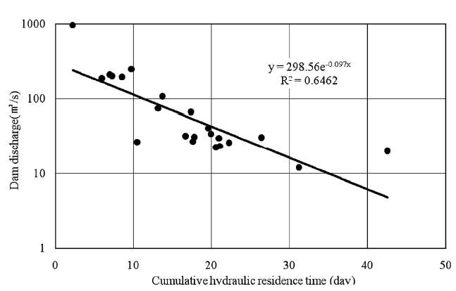
Model prediction errors may be caused by at least three factors.First, errors may be caused by inappropriate representation of the hydraulic characteristics of the study site. Fig. 9 shows the cumulative hydraulic residence time in the study area calculated in QUAL2E. As the figure indicates, there are significant differences in the hydraulic residence time for different dam discharges.The average discharge rate is in the range of 20-100 m3/sec, and this range results in a hydraulic residence time range of 12-27 days. As the depth and width increase in the lower stream area, the residence time also increases. For longer residence times, the model calculates increased reductions in water column concentrations. At times, hydraulic characteristics of the study area can be very complicated due to operation of the Daecheong Dam in the headwater area and the estuarine dam in the downstream area. This is especially true between April and June when flow from the estuarine dam is restricted in order to the raise water levels to provide irrigation water. During this period,the steady flow assumption of QUAL2E is not valid, and special attention must be given when interpreting the results.
In this study, the same hydraulic patterns were assumed for the entire period to compare the two models. If more field data on hydraulic conditions were available, the CAP water quality model could be adjusted to better reflect this situation. In contrast,during the flood season between June and September, the river flow is dominated by discharge from the Daecheong Dam.A significant amount of suspended material is transported due to increased turbidity in the headwaters and resuspension of bottom deposits in the river. The steady state assumption in the hydraulic characteristics, then, may not be valid in this study site for most of the year.
A second source of error may be caused by incomplete specification of pollutant sources. Along the 132 km long river,there may be many unidentified natural or man-made pollution sources. Internal sources can arise in areas of weak currents where pollutants may be deposited. Riverine sediments can release nutrients or other pollutants to the water column when they become anaerobic or when increased flows cause scouring.Dredging for construction material may aggravate this situation.In 2002 and 2003, areas of 1.02 km2 and 1.3 km2, were dredged,respectively, in the study area.
A third source of error is introduced for sampling locations that may not represent the effect of tributaries or point sources effectively. Chapra [14] suggested a required minimum distance for mixing, for side input into a river, as follows:

where, U is the stream velocity (m/sec), B is the stream width(m), and H is the stream depth. If a stream velocity is 0.3 m/sec,width is 100 m, and depth is 2 m, for example, then the required length for mixing is calculated as 12.8 km. It was not always possible to meet this requirement when locating sampling stations due to the length of the river and the accessibility of sampling sites.
The CAP and QUAL2E models were calibrated and applied for 22 consecutive months to 132 km of the Geum River downstream area. The models provided similar predictions for CBOD,COD, TN, and TP when using the same hydraulic, loading and environmental information. The same calibrated decay coefficients were used for PF sections of the CAP model and the equivalent sections in the QUAL2E model. Calibration of the CMF sections in the CAP model, however, led to lower decay coefficients for CBOD and TN, and a higher decay coefficient for TP. Overall, the results demonstrate that the CAP model can treat stagnant reaches separately and can reproduce observed conditions throughout a heterogeneous river successfully.
Nevertheless, significant errors in predictions were found for both models in certain locations and times. These errors are due to three factors:
1) Inaccurate information on hydraulic characteristics, including hydraulic retention time, which affects the amount of pollutant decay.
2) Inaccurate information on external or internal loadings of pollutants.
3) Inappropriate sampling locations and times, which may be affected by insufficient mixing of the river.
This study illustrates results achieved by models of differing kinetic and transport complexity. The choice of model complexity should be based on the objectives of the study and the characteristics of the water body. If a simpler model can provide appropriate results, it should be preferred. The results also demonstrate that accurate physical information, including riverine morphology and flow characteristics, are essential regardless of the water quality model complexity. In this study, only a one dimensional steady state hydraulic model was used. However, dependent on the river conditions being simulated, dynamic characteristics may have to be considered. Finally, non-point source loading due to surface runoff resulting from rainfall may have to be considered in the calculation of average loading.