Inertial measurement units (IMU) consist of gyros and accelerometers. An inertial navigation system (INS) is able to compute its attitude and location using rotation rates and translational accelerations taken from an IMU. Since the INS integrates sensor signals, errors tend to accumulate as time persists. Thus, INS grades vary dramatically depending on the quality of the sensor components. High accuracy systems typically use ring laser gyros or fiber optic gyros. Inexpensive systems, which are widely used for experimental unmanned aerial vehicles, rely on micro-electro-mechanical system(MEMS) components.
Cost effective MEMS gyros and accelerometers present great potential in many areas outside of the aerospace field.However, certain characteristics of MEMS components cannot be easily controlled; such characteristics are susceptible to environmental influences. Because these components are mass produced sold at relatively low prices, manufacturers cannot individually calibrate the components.Consequently, the effectiveness of MEMS based INS becomes limited without appropriately calibrating the sensors.
Sensor fusion is commonly used to improve the accuracy of the INS. By combining a conventional INS with a global positioning system, a magnetometer, and other on-board sensors, users can prevent divergence due to bias from occurring as well as improve the accuracy. However,taking into consideration a worst case scenario in which the supplementary sensors are lost, the importance of the original accuracy of the inertial sensors must be profoundly emphasized.
The conventional method used for calibrating inertial sensors comprises the utilization of rate tables, which consist of gimbals and high accuracy control systems. Users place IMU sensors on top of the innermost table, and they either set the table at a constant angle or drive it at a constant rate.Users calibrate the sensors by comparing the sensor outputs with the reference values of gravity components and angular rates. Such rate tables may be used for HILS (hardware inthe-loop simulation), and are highly priced.
An essential component for calibrating inertial sensors is acquiring the reference rotation rate and acceleration. For calibration only, high accuracy motion control is unnecessary as long as there are reliable reference values.
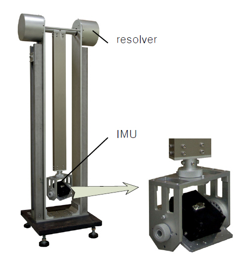
This paper introduces a pendulum based calibration system. The sensors are located at the bob. The movement of pendulum is measured using high accuracy angle sensors such as resolvers or encoders. Based on this angle measurement, rotation rates and accelerations at the sensors are reconstructed. The reference data are then compared to the measurements. Afterwards, the error characteristics of individual sensors are identified.
The authors implemented this and built an experimental setup. This paper will demonstrate the feasibility and usefulness of the method.
2. MEMS IMU and Error Characteristics
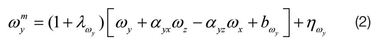
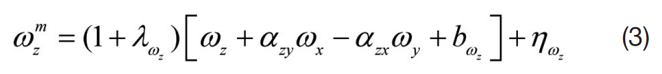
The characteristics of errors vary depending on the sensors. Typical mechanical gyros depend on accelerations in addition to scale and bias errors. Since an IMU consists of 3 or more gyros, alignment errors may also be present.By combining these error sources, measurements acquired from the gyros and accelerometers can be described with the following equations Eqs. (1-6).
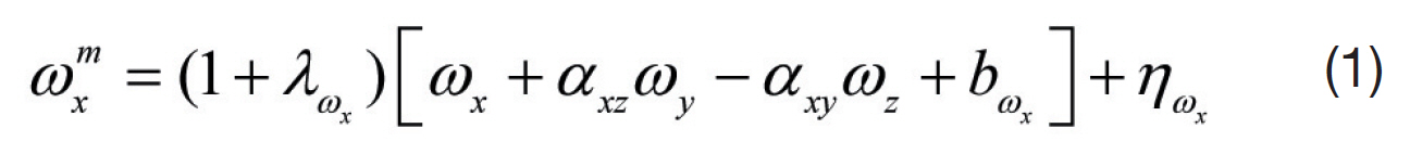
where,
ω
ωi m : measurement of angular rate
λ

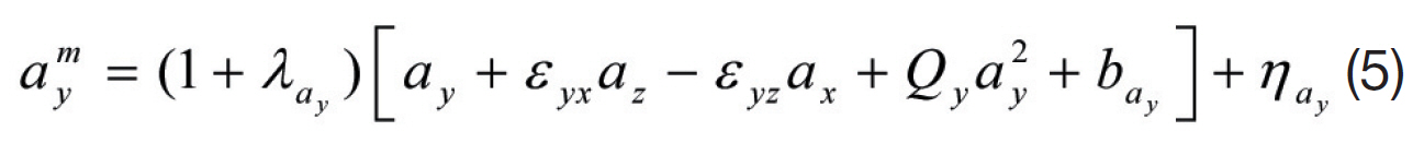

where,
λai : scale factor error ηai : measurement noise
?i : Squared error
The utility of the sensors or IMU becomes fairly limited without accurately identifying the coefficients incorporated in the aforementioned equations.
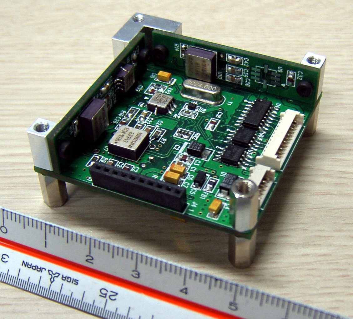
Figure 1 shows an IMU developed by the Aerospace Control and System Laboratory (ACSL) in the Department of Aerospace Engineering, Inha University. The IMU consists of 3 MEMS gyros and 3 MEMS accelerometers. During the system’s first trial, the sensor characteristics varied significantly from component to component. Even identical sets of gyros exhibited drastically different characteristics.This observation led to the conclusion that calibrations must be performed in order to properly utilize the device.
3. Characteristics Calibration Using Pendulum Dynamics
3.1 Acquiring the complete set of data for pendulum motion
The most critical aspect for calibration is acquiring reliable reference data from sources other than the sensors.The conventional method for acquiring reference data is controlling the motion of a rate table with high accuracy. For example, to calibrate a rate gyro, the user places the gyro on a motion table, and rotates the table at a preset speed. Since the motion of the table is controlled with extreme precision,the preset speed can be used as a reference value. The gyro output is compared with the reference speed to find the scale factor and bias.
The whole purpose of the high precision control is to gain reference data. If there is a way to acquire reference data without relying on high precision control, then the expensive control and driving mechanism would not necessary; thus,the cost associated with the calibration process can be significantly reduced.
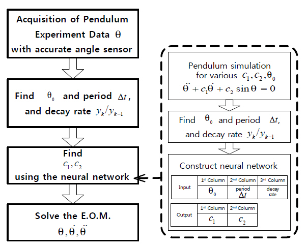
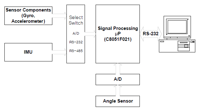
Figure 2 shows a flow chart of a new calibration method that uses reference data acquired from natural pendulum motion.
One dimensional pendulum motion is governed by the following equation of motion.
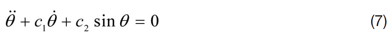
The second term represents damping and the third one is associated with gravity. If angle θ is small, we can use a linear
equation. However, because we need to generate accurate signals for calibration, the equation of motion is considered with nonlinearity of gravity effect.
If one knows the physical coefficients
Figure 3 shows the actual calibration device manufactured by the authors. The sensors to be calibrated are located at the end of the rod. The pendulum angles are measured using a resolver mounted at the rotation hinge. Figure 4 shows the functional diagram of the data acquisition system that is located next to the resolver.
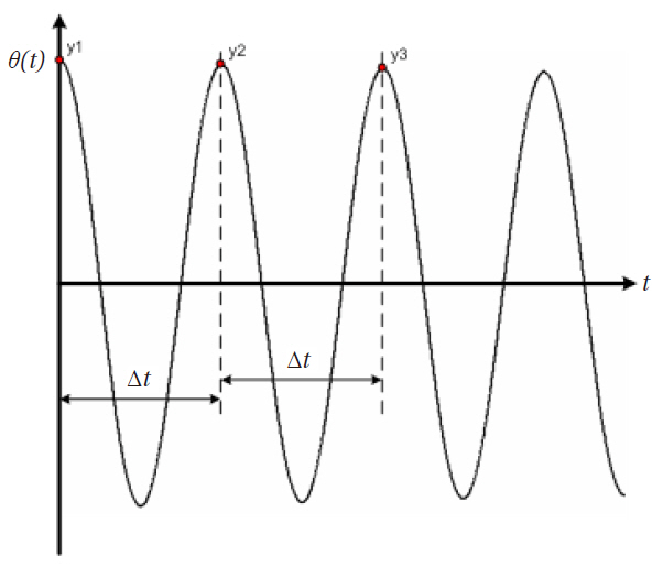
One must find the coefficients and initial conditions to solve the equation of motion. Because the equation of motion is nonlinear, determining the coefficients and initial conditions may be arduous. However, these values are found by using accurate angle measurements from the resolver.The decay rate and period are used to find the coefficients.The initial velocity is set to zero by chopping off the signals before the first peak. Figures 5 and 6 explain this concept.
To find the parameters
In practice, angle measurements using a resolver or an encoder are used for finding θ0, decay rate and period as shown in the left hand side of Fig. 6 Thus, during the experimental investigations, these three values were entered to the neural networks as inputs, and the neural network estimates
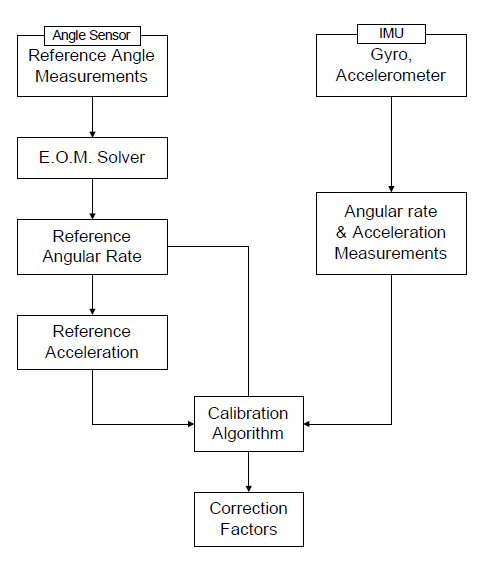
Once the equation of motion was solved, the reference data for the IMU were reconstructed. The single axis pendulum generates signals in 3 degrees of freedom; rotation, tangential acceleration, and normal acceleration.
The terms that contribute to the acceleration are the centrifugal acceleration, tangential acceleration, gravity,and the earth’s rotation. For a rotation with respect to the x-axis, the reference values were reconstructed based on the following formula.
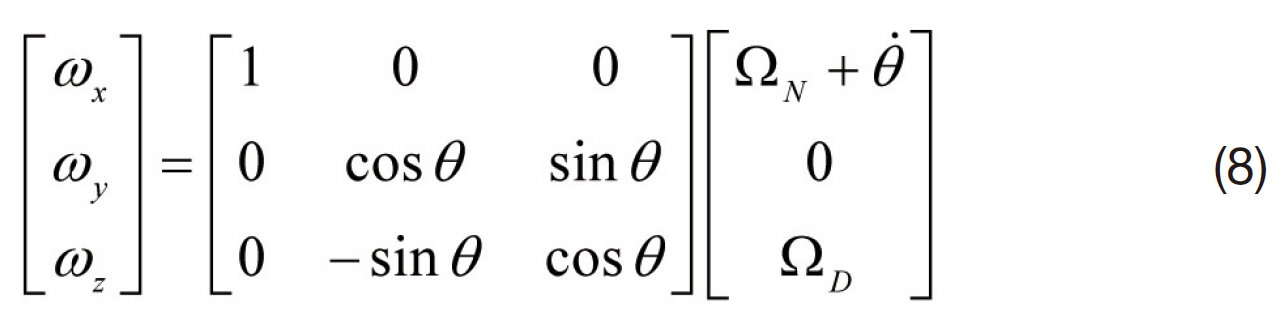
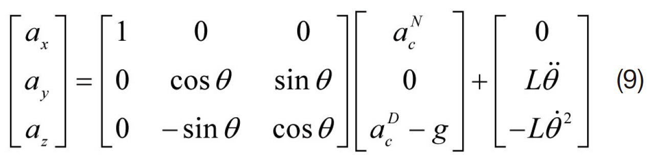
where,
Ω : Earth’s rotational rate
ac : acceleration caused by earth rotation
L : length between sensor and rotation axis
By repeating the procedures 3 times with different orientation settings of the IMU, a complete 6 degrees of freedom reference data are acquired.
Once the reference data set has been constructed, the data was compared to the sensor measurements. The sensor outputs were either in digital or analog. The analog sensor
outputs were digitized using a built-in A/D converter. The measurements were constructed as follows.

where
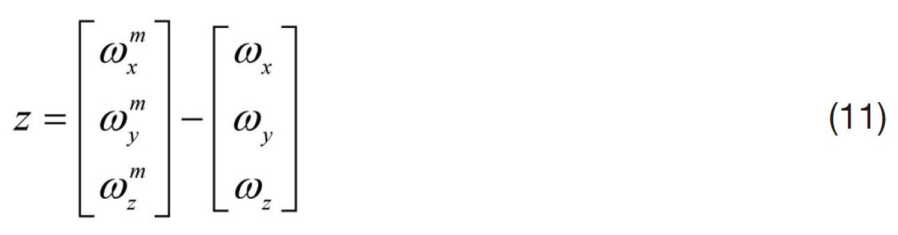
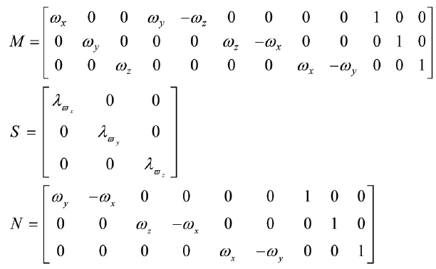
The sensor calibration parameters x?=[
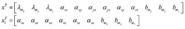
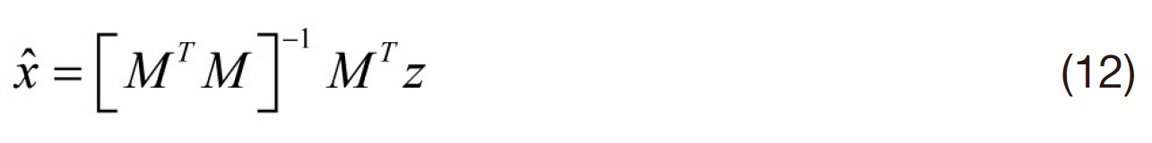
Now, the calibration parameters are identified by solving
The algorithm was implemented and tested with the IMU shown in Fig. 7The first equation to be validated was the equation of motion. Using the resolver measurements,the coefficients and initial condition were identified. Then the equation of motion was solved using these parameters.The resulting angle history was compared to the original measurements.
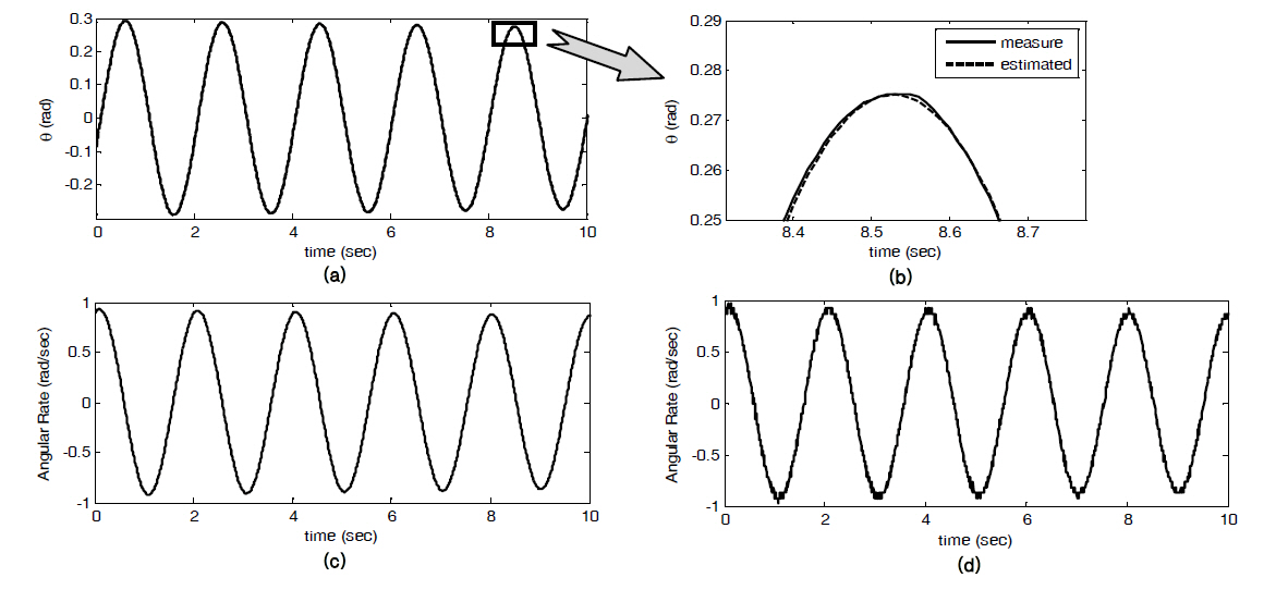
Figures 7a and b show angle measurements and the calculated angle data using estimated parameters of pendulum motion. These angles correlate very well with one another. The enlarged figure (Fig.7 b) proves that the
pendulum obeys the equation of motion well. Since the equation of motion was validated, the angular rate and accelerations that resulted from the equation of motion are considered to be close to the actual rate and accelerations.
Figure 7c shows the angular rate solution. Figure 7d shows the same data computed from numerical differentiation of the angle measurements. Even if the angle measurements appear smooth, the numerical differentiation resulted in significant noise. Differentiating this angular rate resulted in the angular acceleration. However, the results were too noisy and thus deemed ineffective
Using the above validated results, reference data set for IMU calibration was constructed using Eqs. (8 and 9), and
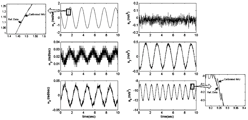
the IMU calibration parameters are identified. Figure 8 shows the 6 sensor measurements along with the reconstructed measurements using the parameters identified in the calibration process. The left side of Fig. 8 shows comparison between calibrated 3-axis angular rate and the reference data. Right side of Fig. 8 shows calibrated 3-axis acceleration and the reference data. The two sets of data match extremely well, which proves the validity of the algorithm.
A new IMU calibration method using a pendulum was devised, and subsequently implemented in a real pendulum system. The reference angular rates and translational accelerations were computed based on measurements from high precision angle measurement.
We constructed the nonlinear pendulum equation,and using this equation the neural network was built for estimating pendulum motion parameters. The angle measurements using accurate angle sensor were entered to neural network as input. After the pendulum motion parameters were estimated, the angular rate and the angular acceleration were calculated using the equation of motion.The acceleration signal, including the Coriolis effect and gravity for calibration, can also be composed by this data.The acquired reference data were compared to the IMU measurements. Consequently, the error characteristics of individual sensors were identified.
This concept was validated with experiments. All the results in this paper prove that calibration of IMU using pendulum motion remarkably improves IMU accuracy.