The Soviet Lunar 2 first succeeded in touching the lunar surface in 1959, and then the USA’s Apollo 11 made the first successful manned lunar landing in 1969. Both countries had performed many lunar exploration missions in the Apollo era, but the competition for lunar exploration decreased after Apollo 17. Since 2000, many countries have again begun programs that will enable them to develop the Moon. Japan,China, and India successfully launched the Selene, the Change’E, and the Chandrayaan-1, respectively, for lunar exploration. There are several reasons to develop the Moon.Helium-3, which is used in nuclear fusion and could be an energy source in the future, is abundant on the Moon, and the existence of water has recently been confirmed by the impact of NASA’s Lunar Crater Observation and Sensing Satellite(LCROSS). In addition, the Moon can be an advance base for reaching other planets. Water will be especially helpful when the lunar base is constructed. Therefore, we need research on lunar exploration so that energy sources can be obtained and the Moon utilized in the development of the other planets.The design of precise trajectories to land at the desired site is very important to making lunar exploration possible, and designs for minimum-fuel, optimal landing trajectories are also needed for spacecraft heavily laden with experimental equipment, as well as to facilitate return of the craft in the event of mission failure. In this paper, trajectory optimization problems are treated so that precise and minimum-fuel landing trajectory, considering the desired landing site, can be designed.

Although many studies of lunar landing were conducted in the Apollo era, the computing power needed to handle the complicated problems was limited, and many assumptions were needed to obtain solutions. Recently,not only has computing power increased to the point where the optimization problem can consider many constraints for practical applications and can therefore be solved, but several numerical methods have also been developed to obtain accurate solutions. Ramanan and Lal (2005) presented several strategies for soft landings from a lunar parking orbit.Tu et al. (2007) have shown how rapid trajectory optimization can be performed for a soft lunar landing using a direct collocation method. Hawkins (2005) treated the trajectory optimization, including the altitude dynamics of the lander,in order to consider the vertical landing. Most of the above studies assumed a transfer orbit phase as a Hohmann transfer or did not consider a landing site. The main contribution of this paper is to generate optimal trajectories from a parking orbit to a specific landing point.

The trajectory optimization problems can be regarded as optimal control problems. To approximate the state and control variables, and the dynamics, a Legendre pseudospectral (PS) method, developed by Fahroo and Ross(2001), was used. In addition, a PS knotting method (Ross and Fahroo, 2004) was applied to handle the multiphase problem because the lunar landing consists of three phases:a de-orbit burn, a transfer orbit phase, and a powered descent phase. After converting the trajectory optimization problem into a finite nonlinear programming (NLP) problem, C code for feasible sequential quadratic programming (CFSQP)(Lawrence et al., 1997) was employed to obtain the optimal solutions.

This paper is organized as follows. The two-dimensional dynamic model is presented in the rotating frame, and the numerical method for the trajectory optimization is reviewed next. The numerical results are discussed, followed by the conclusion.

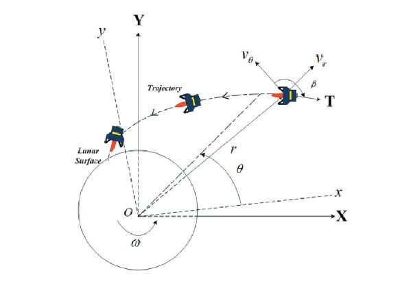
The atmosphere of the moon is extremely thin, so the drag that affects the lunar lander is not taken into account, and the moon is assumed to be a perfect sphere. Because the Moon’s rotation affects the lander’s motion in the rotating frame, the Moon’s angular velocity ω has to be considered,and its value is 2.6632 × 10-6 rad/s. The lunar radius r_m and the standard gravitational parameter μ_m are 1,737.4 km and 4,902.78 km3/s2, respectively. The prime meridian of the moon is the vertical line of the center that is seen from the Earth, and the latitude is zero at the Moon’s equator plane.

In this paper, it is assumed that the landing site is located in the equatorial vicinity of the Moon. Thus, the lander’s motion can be treated as two dimensional. To derive equations of motion, the Moon-centered inertia (MCI)frame and the Moon-centered Moon-fixed (MCMF) frame are needed to represent the relative motion with respect to the rotating frame. If the lander is assumed as a point mass,the equations of the motion in the polar coordinates are derived as follows:

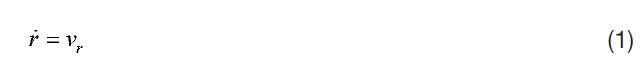
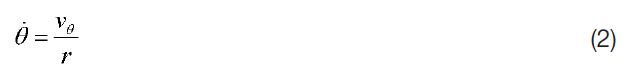
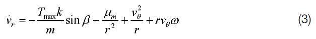
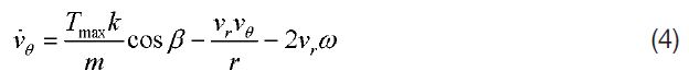
Here, r is the radial position, θ is the center angle, v_r is the vertical velocity, v_θ is the horizontal velocity, g₀ (= 0.00981 km/s²) is the Earth’s gravity, I_sp is the specific impulse, and β is the thrust direction angle. The thrust is calculated by the maximum thrust T_max multiplied by the throttle k, which ranges between 0 and 1.

The trajectory optimization problem can be formulated as an optimal control problem. For solving optimal control problems, there are two major categories: indirect methods and direct methods. In the indirect method, the necessary conditions are used to obtain the optimal solutions, so a complicated calculation is needed. However, the direct method obtains the optimal solutions, minimizing directly the performance index, so the direct method is more useful for a complicated problem because it does not use the necessary conditions (Betts, 1998). In this paper, the direct method is used to handle the lunar landing problems.

A Legendre PS method (Fahroo and Ross, 2001), which has been widely used to solve practical optimal control problems,has been applied to approximate sate variables and control variables, and to state differential equations at nodes called Legendre-Gauss-Lobatto (LGL) points. The lunar landing problem is a multiphase problem because the lander lands on the lunar surface through a de-orbit burn, a transfer orbit phase, and a powered descent phase from a parking orbit.Thus, a PS knotting method (Ross and Fahroo, 2004) has also been applied to perform the trajectory optimization considering all phases of the lunar landing.

After the optimal control problem was converted into the finite NLP problem using the PS method, CFSQP, developed by Lawrence et al. (1997) at the University of Maryland, was used to obtain optimal solutions. CFSQP is a numerical solver using a SQP algorithm.

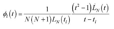
Collocation methods usually use piecewise-continuous functions to approximate the state and control variables on the arbitrary subintervals. However, the Legendre PS method uses globally interpolating Lagrange polynomials as trial functions for approximating the state and control variables at the LGL points. The LGL points are the zeros of the derivative of the Legendre polynomial L_N except for the end points (t₀ =？1, t_f = 1), and they lie in the interval [？1, 1], so the following transformation is needed to express the problem in the LGL time domain (t∈[t₀, t_N] = [？1, 1]):

The continuous variables are approximated by N-th order Lagrange polynomials ø l (t).

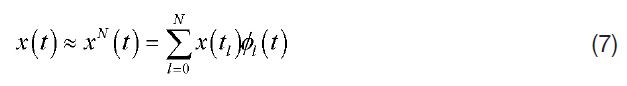
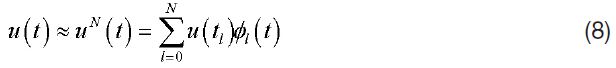
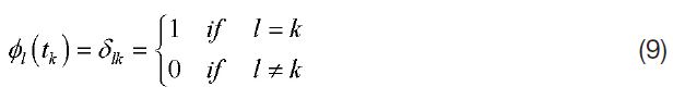
where for l = 0, 1, ..., N

It can be shown as the Kronecker delta function that

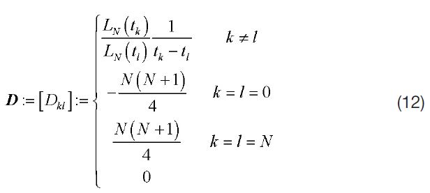
The state differential equations are transformed into the algebraic equations using the PS differentiation matrix D:

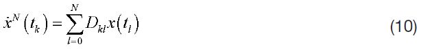
where

The performance index can be discretized using the Gauss-Lobatto integration rule:

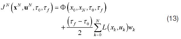
where

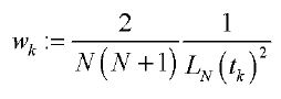
and w_k are the LGL weights given by

To solve multiphase problems, many nodes are needed for accurate solutions to be obtained; this requires a great deal of computation time. In this case, using the PS knotting method, those problems can be solved efficiently with fewer nodes. The basic idea of the PS knotting methods is to divide the whole time interval into smaller subintervals when the time histories of the states and/or controls have large variations. Then, the double LGL points, called knots,are placed between the subintervals, and the Legendre PS method is applied to discretize each phase. There are two kinds of knots. A soft knot is one located at a place where the state values are continuous and the control values are discontinuous between the subintervals. A hard knot is one located where the state values are discontinuous between subintervals.

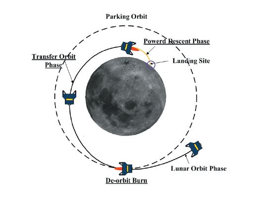
A lunar landing consists of three phases: a de-orbit burn,a transfer orbit phase, and a powered descent phase. The deorbit burn enables the craft to enter the transfer orbit phase,which is an elliptical orbit (100 × 15 km), from a parking orbit; then the lander descends without thrust during the transfer orbit phase. The perilune height of 15 km is chosen to minimize fuel consumption and in consideration of the mountainous terrain of the Moon and possible guidance errors (Bennett and Price, 1964). The powered descent phase is initiated near the perilune when the engine turns on, and the lander’s velocity is totally decreased in order to enable the craft to land softly on the lunar surface.

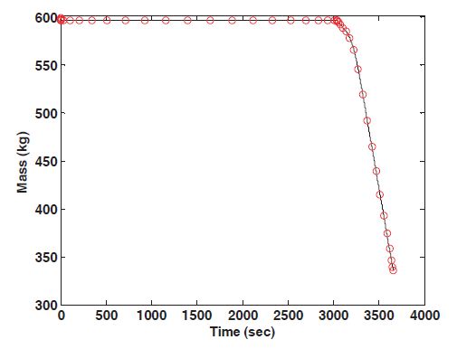
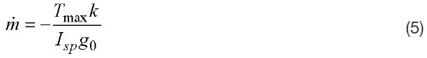
In the parking orbit the initial mass m₀, the specific impulse I_sp, and the maximum thrust T_max are 600 kg, 316 seconds, and 1,700 N, respectively.

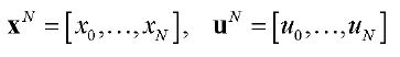
The state and control variables are defined as

The lander has to minimize fuel consumption if it is to carry a heavy payload of mission equipment for lunar explorations and to be able to return in the event that the mission cannot be completed. Thus, the performance index is defined so as to minimize the lander’s fuel consumption:

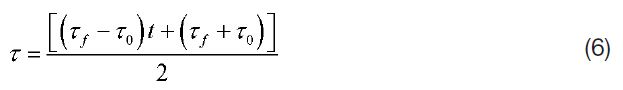
For the optimization results to be obtained officially, the NLP variables should be of a similar order of magnitude.Thus, it is necessary to normalize them using the following scaling factors:

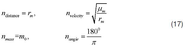
Using the above scaling factors, time τ, specific impulse I_sp,the Earth’s gravity g₀, the Moon’s angular velocity ω, thrust T_max, and the standard gravitational parameter of the Moon μ_m can be normalized.

The NLP variables, which are obtained from the optimization results, are

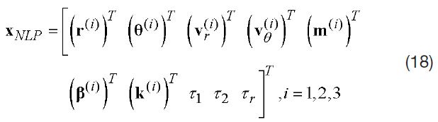
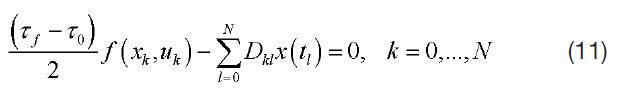
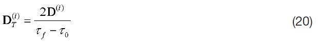
where i = 1, 2, 3 represent the de-orbit burn, the transfer orbit phase, and the powered descent phase, respectively.Constraints imposed when the optimization is performed consist of the dynamic, initial, terminal, and event constraints.From the equations of motion, the dynamic constraints are defined as

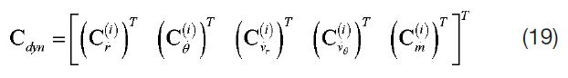
where

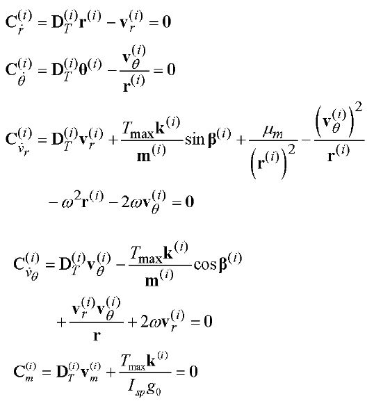
and D_T⁽ⁱ⁾ is defined as

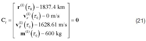
The initial altitude is 100 km from the lunar surface. The initial vertical velocity is zero in the parking orbit, and the horizontal velocity, which is the velocity relative to the MCMF frame, is calculated by the difference between the circular velocity

and the velocity (ωr(τ₀)) caused by the Moon’s rotation. The center angle is one of the parameters that represent the lander’s location. Thus, the initial center angle should be found from the optimization result because the optimal trajectory to land at the designated landing point is changed as the initial location of the lander changes.Therefore, the total initial constraints are

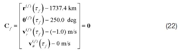
The terminal altitude is the surface of the Moon, and the terminal velocities are determined for soft landing. The landing site is determined by the terminal center angle because the downrange is calculated by multiplying the lunar radius and the change in center angle. The terminal center angle is 250 deg and arbitrarily determined as the desired landing site. Hence, the terminal constraints are given by

To connect the state or control information between each phase, the knotting constraints are needed as follows:

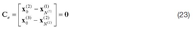
where x⁽¹⁾, x⁽²⁾, and x⁽³⁾ denote the first, second, and third phase state variables, respectively, and the subscript means the N-th variable. In addition, the time constraints are imposed as follows:

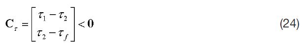
The terminal constraint of the de-orbit burn is needed in order to enter the transfer orbit phase [3].

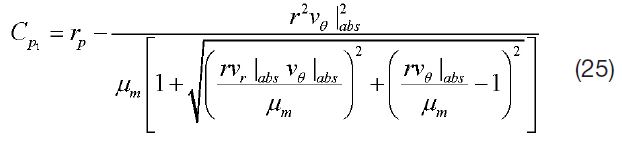
where v_r│_abs and v_θ│_abs are the absolute velocity. In Eq. (25),r_p is the perilune height, and the shape of the transfer orbit is determined by r_p at the terminal time of the de-orbit burn,which means that if r_p is 15 km, the de-orbit burn forms the 100 × 15 km transfer orbit phase.

The constraint on the termination of the transfer orbit phase is also needed to start the powered descent phase.

If the inequality constraint of Eq. (26) has a much lower value, the landing problem can be either infeasible or overly constrained.

A throttle bound is defined to avoid restarting of the engine during the powered descent phase:

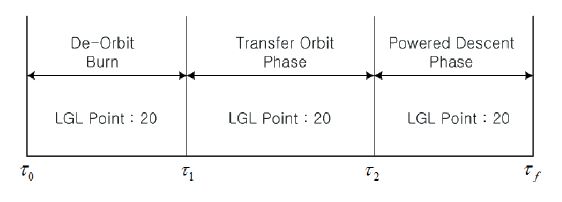
In Fig. 3,the total number of the LGL points is 60, and each phase has LGL points of 20. Although the transfer orbit phase has longer duration than the other two phases, setting the LGL point to 20 in the transfer orbit phase is allowable because the control variables are not computed during freefall descent, and only the integration is only performed.

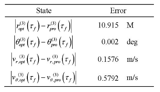
A feasibility check is performed in order to verify the optimization results. Feasibility means that the control and path constraints, the boundary conditions, and the dynamics constraints are satisfied (Josselyn and Ross, 2003).Feasibility can be checked by verification of whether the time histories of the states obtained by the propagation using the controls obtained from the optimization results match the state values obtained from the optimization at the LGL points. To propagate the states from the initial conditions,the control values obtained from the optimization at the LGL points need to be interpolated. Thus, the cubic interpolation scheme is used to interpolate the control values, and fourthorder Runge-Kutta method is used to propagate the states from the initial conditions. Table 1 shows the terminal

propagation errors of each state. In Hawkins (2005), the terminal propagation error of the altitude is about 100 meters when all landing phases from the parking orbit are considered, so it is deduced that the results obtained in this paper are good solutions. If more LGL points are used, more accurate solutions can be obtained, and there will be fewer propagation errors.

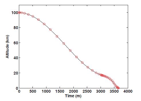
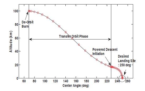
Figures 4 through 11 show the trajectory optimization results, and the circles and the solid lines represent the optimized and propagated values, respectively. Figure 4 represents the two-dimensional trajectory from the optimized initial location (69.29 deg) to the desired landing (250.0 deg)site. The lander travels downrange 5,479.8 km from the initial location, and a total flight time of 3,655.3 seconds is taken for

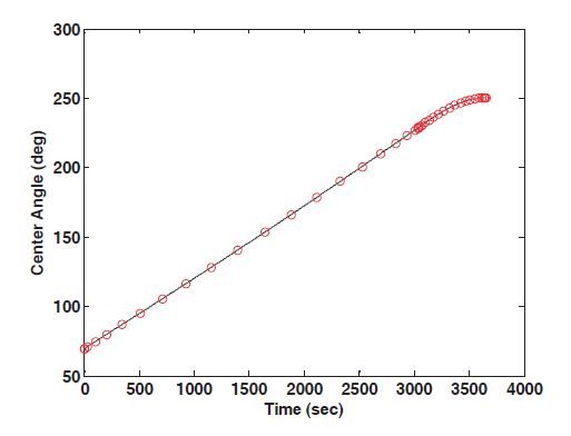
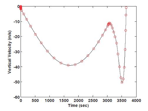
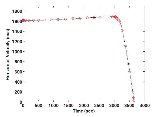
the landing at the desired site. Figures 5 and 6 show the time histories of the altitude and the center angle. The duration of the de-orbit burn, the transfer orbit phase, and the powered descent phase are 6.90 seconds, 3,028.5 seconds, and 619.98 seconds, respectively. The velocity profiles are shown in Figs.7 and 8, and the terminal constraints are satisfied for a soft landing. Figure 9 represents the lander’s mass profile, and the fuel consumption of the de-orbit burn and the powered descent phase are 3.768 kg and 260.69 kg, respectively. In Fig. 10,the lander’s engine turns on at the altitude of 17.009 km

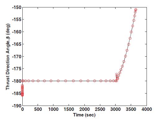
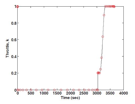
when the powered descent phase is entered, and the throttle is full about 300 seconds after entering the powered descent phase. The time that the engine turns on can be controlled by changing the termination altitude of the transfer orbit phase in Eq. (26). In Fig. 11, the thrust direction is opposite to the lander’s motion in order to reduce the velocity and change almost linearly from -180 deg to -151 deg during the powered descent phase.

This paper is concerned with two-dimensional trajectory optimization for a soft lunar landing, at a desired landing site.To discretize the continuous trajectory optimization problem,the PS method was applied, and CFSQP was used to obtain the optimal solutions. The constraint on the terminal center angle was imposed to consider the desired landing site, and the initial center angle was obtained from the optimization results because the optimal trajectory can be changed as the initial location changes. All constraints on the states and controls are satisfied, and although propagation errors appear, they can be reduced if more LGL points are allocated at each phase. Through the trajectory optimization problem dealt with in this paper, it is expected that more precise lunar landing trajectories can be generated for future lunar exploration.