Most aircrafts developed before the 1980s have hydromechanical systems, the control surfaces and hydraulic systems of which are connected by mechanical hinges. This type of system requires great effort from the pilot to control the aircraft, and the aircraft itself is robust in the face of environmental changes. Because of these properties of hydro mechanical system, it is hard to maintain full control for a while. The fly-by-wire (FBW) system was developed in an effort to solve such problems. In the FBW system, electric devices are used in place of mechanical systems. The flight control computer (FCC) receives a sensor signal and sends commands directly to the control surface. Usage of the FBW system improves aircraft system controllability, comfort, and safety.

With the development of FBW technique, the performance and handling quality issues associated with flight envelope limits have driven the need for a carefree maneuvering capability. As such, the concept of flight envelope protection has been actively studied (Airworthiness Performance Evaluation and Certification Committee, 1999; Horn and Sahani, 2004; Howitt, 1995; Sahani, 2005; Whalley and Achache, 1996; Wilborn and Foster, 2004; Yavrucuk et al., 2009).The flight envelope protection system predicts the aircraft state in the near future time and generates a control signal to the actuators to prevent the aircraft from exceeding the flight envelope. This system has many benefits, including preventing the aircraft from exceeding its structural/aerodynamic limits and its control surface saturation and decreasing the mission time by allowing for maximal panel monitoring. Because of these benefits, many modern aircrafts are equipped with the flight envelope protection system.

There are several flight envelope protection schemes,including the fixed horizon prediction, the dynamic trim algorithm, the peak response estimation, and the adaptive neural network-based algorithm (Sahani, 2005). In this study,the flight envelope protection system is designed using the dynamic trim concept. In the fixed horizon prediction scheme, the target state value is predicted after a fixed amount of time. To achieve this, a functional relationship with the state value, control inputs, and fixed time step (prediction horizon) is used. If the critical parameter is expected to reach its limit value in the future, the protection algorithm works to protect the critical parameter from exceeding its limit value.The dynamic trim algorithm is a prediction algorithm that uses the dynamic trim concept, a quasi-steady maneuvering flight condition. Aircraft states are either fast or slow: fast states are the flight parameters that achieve a steady state in dynamic trim, while slow states vary during the dynamic trim. Therefore, only the slow states can be used to estimate the critical parameter. The neural network is generally used to correct errors between the real system and the estimated system. The peak response estimation scheme is designed to estimate the transient peak of the critical parameter that occurs immediately after the control input. This algorithm predicts a very near term response of the critical parameter.Hence, a linear model of the fast dynamics can be used.The adaptive neural network-based algorithm is similar to the dynamic trim algorithm. It uses the dynamic trim assumption and also uses the adaptive neural network to predict the critical parameter value (Sahani, 2005).

A flight envelope protection system using dynamic trim is designed in this study. The dynamic trim algorithm is very efficient because of its simple structure. However, it ignores differential terms; therefore, it includes come errors. To reduce this error, the 1st derivative term is introduced in this study. The modified dynamic trim algorithm has better performance than the conventional dynamic trim algorithm.To verify the performance of the proposed algorithm, the results of the proposed method are compared with these of the peak response estimation.

This paper is organized as follows. In Section 2, the concepts of the flight envelope and the loss of control are introduced. The flight envelope protection system structures and the limit avoidance algorithms are presented in Section 3. In Section 4, the numerical simulation results are shown.Finally, conclusions are addressed in Section 5.

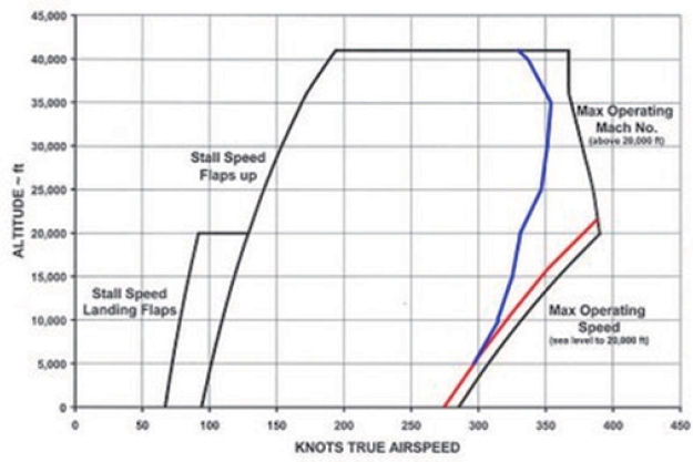
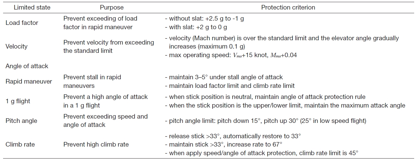
The flight envelope is defined as the territory in which the aircraft can fly safely inside various limits. The flight envelope is defined by Mach number, altitude, limited load coefficient,and other variables. The envelope boundary is related to the aircraft stall limit, thrust limit, and structure limit. Figure 1 shows the typical example of the flight envelope of Eclipse 500, while Table 1 shows the flight envelope protection rule.

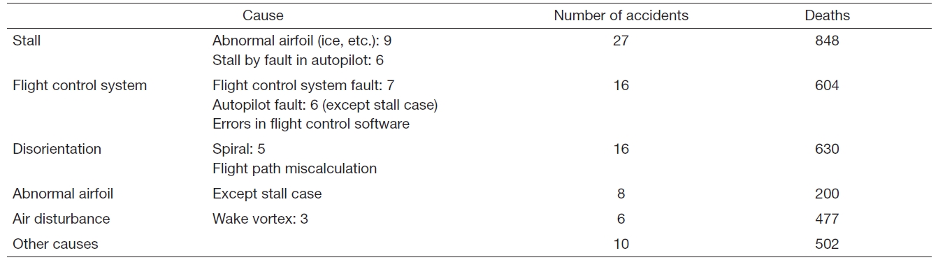
Loss of control is the state in which the aircraft exceeds the flight envelope and the pilot cannot control the aircraft using stick input. The main causes of this state include stall,roll by sideslip angle, pilot-induced oscillation, and yaw. In the loss of control state, the aircraft may become unstable and accidents may occur (Wilborn and Foster, 2004). Table 2 shows the accident cases in civil aircraft systems due to loss of control. Most of the accidents occurred in aircraft that did not have the flight envelope protection system. These results suggest that use of the flight envelope protection system is required to reduce the accident rate.

The flight envelope protection system is designed to generate a control signal when the aircraft is expected to exceed the flight envelope limit. The critical parameters are the variables that are closely related to the flight envelope that must be restricted. When a critical parameter is over the limit value, loss of control may occur. Critical parameters include angle of attack, speed, climb rate, load factor, and pitch angle. Let us define a parameter vector as y_p and its limit values as y_lim and y_lim. The flight envelope protection problem is defined as the problem of finding the control input that satisfies the following equation.

The flight envelope protection system consists of a limit prediction component and a signal generation component.The limit prediction component uses the current flight state,pilot’s input, and flight envelope to estimate the lower and upper input values that will make the critical parameters exceed the limit value. Use of the limit prediction algorithm is required to achieve this. The signal generation component generates a signal using the estimated limit values in the limit prediction component of the flight envelope protection.Two flight envelope protection methods are widely used:the hard envelope protection method and the soft envelope protection method (Yavrucuk et al., 2009).

3.2.1 Hard envelope protection

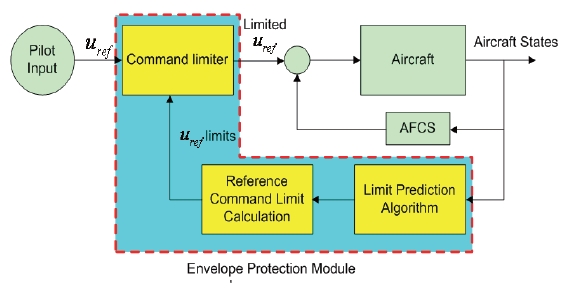
In the hard envelope protection scheme, the control input is generated by comparison of the critical input and the pilot’s input. If the aircraft nears flight envelope escape, the protection scheme sends a control input directly to the FCC.This structure recognizes the approaching flight envelope exceeding situation and yields more efficient performance than the soft envelope protection scheme by directly adjusting the control input. Figure 2 shows the structure of the hard envelope protection system in which the command limiter works as the signal generator (Airworthiness Performance Evaluation and Certification Committee, 1999).

3.2.2 Soft envelope protection

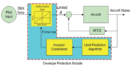
The soft envelope protection scheme generates warning signals including visual signals, sounds, and stick force.By observing these signals, the pilot can recognize that the aircraft is nearly exceeding the flight envelope and change the control input for the envelope protection. According to National Aeronautics and Space Administration research,auditory or visual warnings cannot make the pilot recognize the light condition fast enough to act properly for protection.Therefore, the pilot usually overacts and provides excessive control input that makes the aircraft unstable. On the other hand, the pilot can quickly recognize the flight condition when the active stick force cue is used to issue the warning signal. Figure 3 shows the soft envelope protection scheme in which the active stick force cue generation component is in the envelope protection module instead of the command limiter (Airworthiness Performance Evaluation and Certification Committee, 1999).

3.2.3 Limit avoidance algorithm

Critical values must be predicted to make aircraft fly safely inside the flight envelope. Limit avoidance algorithms are widely used to predict the flight state. There are several limit avoidance algorithms, including fixed horizon prediction,dynamic trim algorithm, peak response estimation, and adaptive neural network-based algorithm (Sahani, 2005). The fixed horizon prediction method calculates the prediction horizon, a fixed time in which the limit parameter is expected to reach its peak value. The following approximated system is used to estimate the protection horizon value.

A neural network is used to determine the coefficients of function f (x, u, t).

The dynamic trim algorithm uses the concept of “dynamic trim” to calculate the critical input. In the dynamic trim algorithm, a quasi-steady flight condition is assumed and the aircraft states are divided into fast and slow states. The fast states have relatively quick dynamics; therefore, they

comprise the steady state in the dynamic trim condition. The dynamic trim condition corresponds to the flight condition in which the fast states are in the equilibrium states as follows.

where x_f denotes the fast state variables. Using Eq. (3),the aircraft response in the quasi-steady flight condition can be expressed in terms of the slow states and the control input. Because the fast state variables are not changed, the following approximate dynamics of the aircraft can be used to calculate the critical input.

where x_s denotes the slow states.

Peak response estimation is used to predict the transient peak of the response. This algorithm predicts the short-term response of the limited parameter. Therefore, a linearized system for the current flight condition is needed to calculate the critical input. An analytical solution can be found in the linear model; therefore, the peak response estimation algorithm is very efficient.

The adaptive neural network-based algorithm uses the dynamic trim concept and an adaptive neural network to make the critical input computation. In this scheme,the approximated system is first constructed using the dynamic trim concept. The estimation errors between the approximated system and the real aircraft dynamics are then estimated using the adaptive neural network. The algebraic equation set can be obtained through this process, and the critical input can then be computed by solving the obtained algebraic equation.

In this paper, the dynamic trim concept is adopted to design the flight envelope protection system, and it is modified to accurately estimate the critical value.

The term “dynamic trim” refers to a quasi-steady maneuvering flight condition. In the dynamic trim condition,it is assumed that the states with fast dynamics are converged to create the steady value. Aircraft equations of motion can be represented as

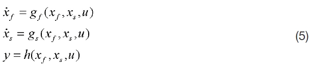
where x_f is a fast state vector, x_s is a slow state vector, u is a pilot control input vector, and y is the protection parameter.

The dynamic trim condition can be represented as

Using Eq. (6) in Eq. (5), we have

As shown in Eq. (7), flight parameter can be considered as a function of slow states and a control input. Note that the approximate function h(x_s, u) is very important in the prediction of a critical value. In this study, it is assumed that the critical states are variables among the state variables,meaning that y can be written as

Let us consider the linearized system

Using Eqs. (8) and (9), the following equation can be obtained.

The steady state condition of the critical states is used in the conventional Dynamic trim algorithm. In this study,instead of the steady state condition, the finite difference relation is used to modify the dynamic trim algorithm as

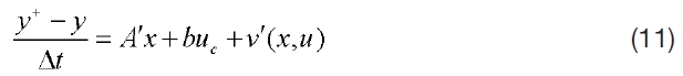
where y⁺ denotes the value of target parameter in the near future, u_c is the control input used to protect the target parameter y, and v'(x, u) is the difference between the approximated polynomial function and the real aircraft dynamics. A neural network is used to estimate the value of the high order term v'(x, u). The neural network inputs

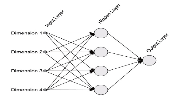
include the flight states and the control input. Figure 4 shows the structure of the single-layer neural network used in this study.

The upper and lower critical control inputs can be obtained by using Eq. (11) as

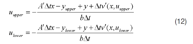
where y_upper is the upper critical limit and y_lower is the lower critical limit. As shown in Eq. (12), the critical input terms exist on both sides of the equations; therefore, an iteration technique is used to find a solution.

The conventional dynamic trim algorithm cannot be applied to state variables that cannot be directly controlled by pilot input, including pitch angle and angle of attack. In this study, the dynamic trim algorithm is modified to apply a system in which the target parameter is indirectly controlled by a variable that is closely related to the target parameter.Let us consider a variable that satisfies the following equation with the target parameter:

where f(y) is a non-singular continuous function. For the critical limit of target parameter y_crit and the value of z_crit corresponding to Eq. (12), the relation of y_crit and z_crit can be expressed as follows:

The critical input to prevent exceeding of the critical limit z_crit can be obtained as:

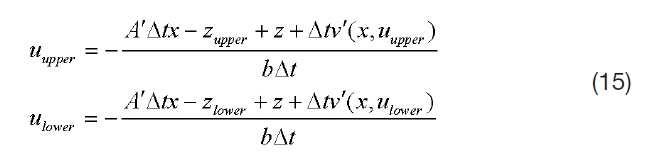
Substituting Eq. (14) into Eq. (15), we have:

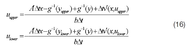
The above equations can be used to protect the state variables that cannot be directly controlled by pilot input. In this paper, the algorithm is also applied in a case in which multiple variables are the target parameters for protection.The following logic is used to protect the multiple target parameter case.

I. Choose a control input that has the most effective target parameter. Construct a pair of control inputs and parameters including throttle speed, elevator pitch, etc.

II. Rank the priority of critical input calculation. Variables that cannot be controlled directly by the pilot’s control input are considered first. The variable that does not have steady state response critical limits has priority.

III. Apply the dynamic trim algorithm sequentially according to priority.

The peak response estimation algorithm is used to find the transient response. This algorithm estimates the value using the short-term interval; therefore, a linearized system can be used to calculate the critical input. Approximate aircraft dynamics of single input-single output linear systems can be expressed as follows:

where Δx = x ? x_e, Δy = y ? y_e, and Δu = u ? u_e. For a nonzero initial value, the step response of the system can be expressed as:

Using the initial output value, Eq. (18) can be expressed as:

where y₀ = y(0) = y_e + CΔx_o, E₁(t) = C(e^At ? I),

and E² = CA^?1(e^At ?I)B. The norm of Eq. (9) can be written as:

where F = E₂ ^TE₂, G = 2(Δx₀ ^T E₁ ^T + y₀ ^T)E₂, and H = y₀ ^T y₀ + 2y₀ ^T E₁Δx₀ + Δx₀ ^T E₁ ^T E₁Δx₀. The value of y(t) can be estimated using Eq. (20).

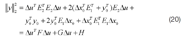
For the input vector u = [δ_long δ_lat]^T, Eq. (20) can be represented as an ellipse on the plane composed of δ_long andδ_lat (Fig. 5). This ellipse demonstrates the boundary of the stick position that makes the output not exceed the limit value at the given time. Note that E¹ and E₂ values can be calculated in advance; therefore, F, G, H can be quickly calculated using the set of pre-computed E₁ and E₂ values.

Equation (20) can be rewritten using a scalar variable d as:

where d is the distance between the given input and the critical input and n is a gradient vector defined as

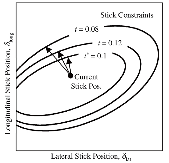
The critical control margin vector Δu* is the minimum distance between the current control input and the critical input. It can be expressed as

where d* = min(d). In this way, the critical input can be computed using d*(Airworthiness Performance Evaluation and Certification Committee, 1999).

In this study, the conventional algorithm is modified to handle multiple-variable cases for protection as follows:

Calculate the threshold distance d* on each target parameter by solving Eq. (21) as:

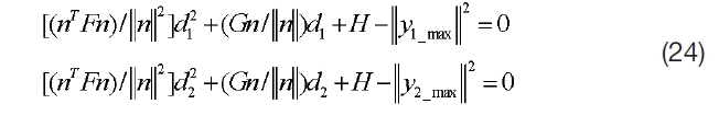
Among the threshold values, select the minimum distance as:

Calculate the critical control margin vector Δu* using d*_s as:

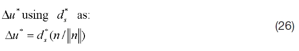
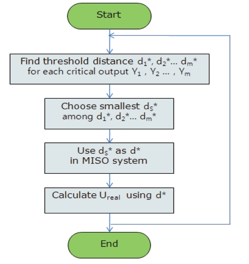
Figure 6 shows procedure for MIMO case problem. This procedure is additional step to expand algorithm from SISO to MIMO. Procedure for SISO case is explained in Eqs. (17)-(23). The peak response estimation algorithm uses all of the control inputs to protect one target parameter. Therefore, the closest parameter to the critical limit should be considered first.

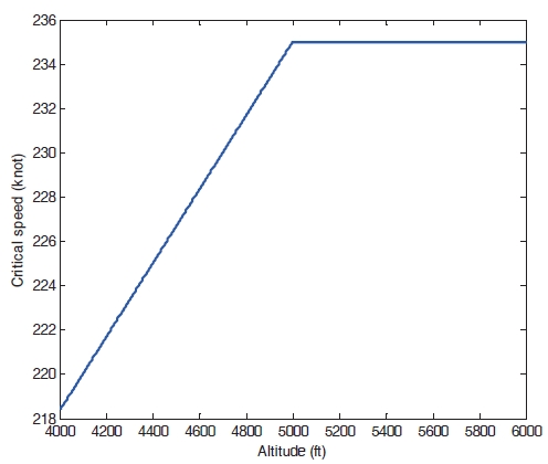
In this section, numerical simulations are performed to verify the performance of the proposed algorithm. For the numerical simulation, the Eclipse 500 non-linear dynamic model is considered. The flight envelope protection algorithm is applied to restrict the body speed and pitch angle. Critical speed value is dependent on the altitude. Figure 7 shows the critical speed considered in this study. The upper and lower limits of the pitch angle are ±5°, respectively.

From the motion equation, it can be observed that the pitch angle cannot be directly controlled by the pilot input.Instead, the pitch angle can be indirectly controlled through control of the pitch rate, which can be directly controlled by the elevator input. Therefore, let us set the critical limit of the pitch rate to prevent the pitch angle from exceeding the limit as follows:

where k and a are arbitrary positive values of the margin.When the pitch angle approaches the upper limit, the control input should make the aircraft pitch down and vice versa.The equation of the pitch rate can be written as follows:

where (a, b, c, d, e, f, g) are the coefficients related to the aerodynamic and control derivatives, x is the aircraft states (u, w, q, θ), and δ is the control input (δ_ele, δ_th, δ_rud, δ_fr).Consider the error dynamics of pitch rate as:

Using Eq. (27) and Eq. (28), the error dynamics equation can be written as follows:

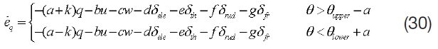
Error can be converged to zero by satisfying the following relationship:

where α is an arbitrary positive value. Using Eq. (30) and Eq. (31), the critical value of the elevator control can be computed as:

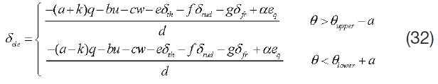
Now let us consider the following performance indices to verify performance of the proposed algorithm:

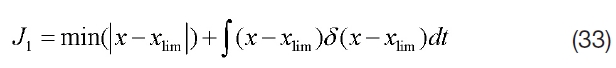
where J₁ is the sum of the minimum distance between target parameter and critical limit and the area exceeding the critical limit. J₁ represents the closeness to the critical limits; therefore, it can be considered as the performance of the envelope protection. J₂ is the maximum value of the differential of critical control input, which represents the rate of critical input changes. In this study, 2 control inputs comprise the pilot’s command inputs.

Case 1)

Throttle input: constant step input

Elevator input: constant step input

Case 2)

Throttle input: pulse input

Elevator input: constant step input

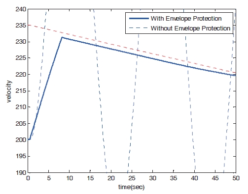
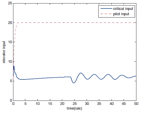
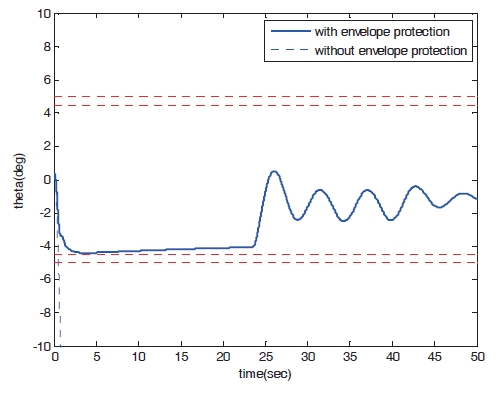
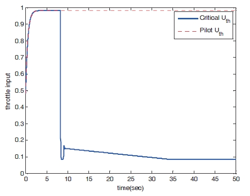
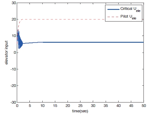
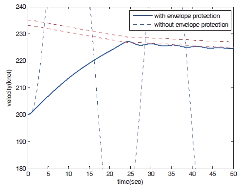
Figures 8?11 show the numerical simulation results of the dynamic trim algorithm for Case 1. As the throttle input reaches the maximum value using to the pilot’s input, the speed increases and approaches the critical limit. To prevent exceeding the upper limit speed, the critical throttle input value decreases (Fig.8 ). As shown in Fig. 11,the pitch angle is also protected.

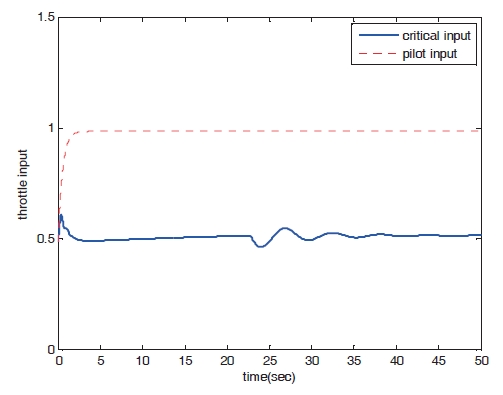
Figures 12?15 show the numerical simulation results of

the peak response estimation algorithm for Case 1. Pitch angle quickly approaches the critical limit and the throttle and elevator input change simultaneously. As shown in Fig.13, the speed of the peak response estimation algorithm increases less quickly than that of the proposed dynamic trim algorithm.

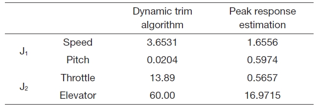
Table 3 summarizes the performance index values. As shown by the J₁ values, the peak response estimation speed

is larger than that of dynamic trim algorithm. However, the pitch angle of the dynamic trim algorithm is smaller than that of peak response estimation. As shown by the J₂ values,the critical inputs of the dynamic trim algorithm change more rapidly and largely than those of the peak response estimation.

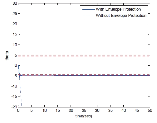
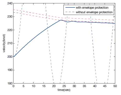
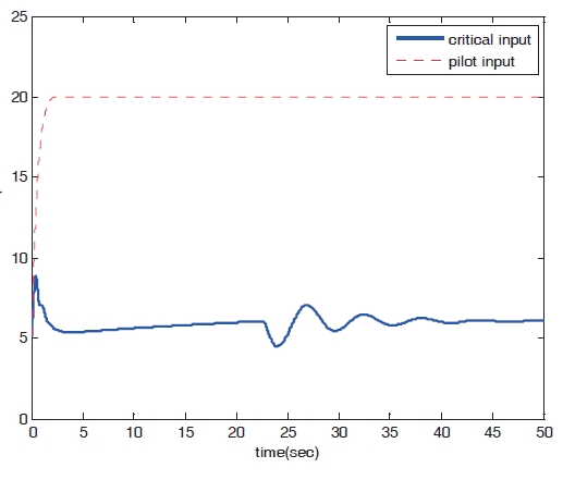
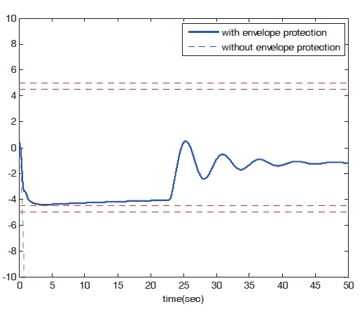
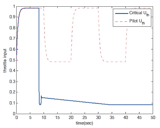
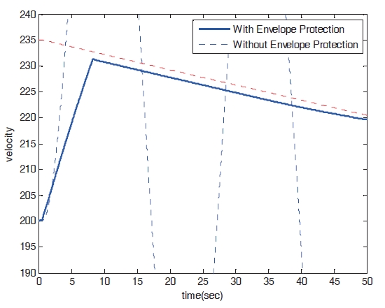
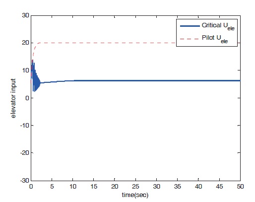
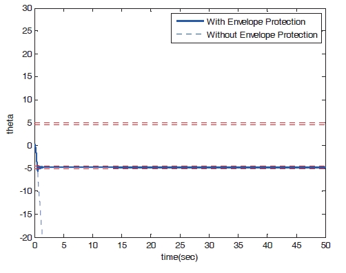
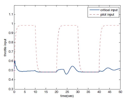
Figures 16?19 show the results of numerical simulation of the dynamic trim algorithm for Case 2. Similar to the results of Case 1, the speed increases and approaches the critical limit. To prevent the speed from exceeding the upper limit,the critical throttle input value then decreases (Fig.16 ). After the speed approaches the critical limit, the control input variables and states show patterns similar to those of Case 1.

Figures 20?23 show the numerical simulation results of the peak response estimation algorithm for Case 2. The results are similar to those of Case 1; however, the elevator input and pitch angle are not converged to create steady state values.

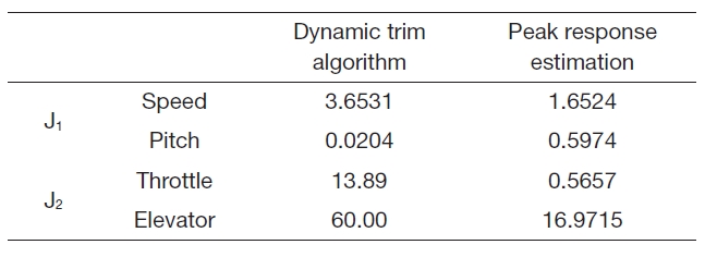
Table 4 summarizes the performance index values and shows that the J₁ and J₂ trends are the same as those of Case 1. This result is caused by the pilot’s control input exceeding the critical control.

In this study, a flight envelope protection system is designed using the dynamic trim algorithm. To improve the algorithm’s accuracy, the critical input computation equation is modified by considering the first derivative of the critical value. The flight envelope protection algorithm is also expanded to handle multiple target parameters. Numerical simulation is performed to verify the algorithm performance.The results of the proposed method are compared with those of the peak response estimation algorithm. The dynamic trim algorithm has better flight envelope protection performance than does peak response estimation. However, the critical input of the dynamic trim algorithm changes rapidly when the target parameter approaches the critical limit. Further studies are required to handle this problem.