Reduced weight, increased structural flexibility and operating speed certainly increase the likelihood of flutter occurring within the aircraft operational envelope. The mission profiles of next generation of flying vehicles will require adaptable airframes to best meet varying flight conditions. However, geometry changes could possibly incur aeroelastic instabilities, such as flutter, at transition points during the mission. New requirements imposed on the design next generation vehicles have called for increasing structural flexibility, and high maneuverability while maintaining the ability to operate safely in severe environmental conditions. Consequently, developing and implementing active control technology has become very important. In the last two decades, the advances in active control technology have rendered the applications of active flutter suppression and active vibrations control systems feasible. Great research efforts are currently devoted to the aeroelastic active control and flutter suppression of flight vehicles. Librescu and Marzocca (2005) presented state-ofthe-art advances in these areas. Recent contributions related to the active control of an aircraft wing are discussed in length in a publication by Mukhopadhyay (2000a, b, 2011).
Behal et al. (2006b), Guijjula et al. (2005), Plantantis and Srganac (2004) presented novel research that improved the performance of adaptive schemes through wing extensions containing two control surfaces. Platanitis and Strganac(2004) presented an adaptive scheme that utilized fullstate feedback. However, the uncertainty in the coupling between the control inputs was not taken into account.Rather, an inversion of the nominal input gain matrix was utilized to decouple the control inputs. Gujjula et al. (2005)designed adaptive and radial basis functions neural network controllers in order to compensate for system nonlinearity.Furthermore, a projection operator was utilized to assure that the input gain matrix estimate remained invertible.To sidestep the need for projection, Behal et al. (2006b)utilized a symmetric-triangular decomposition of the input gain matrix in order to design singularity free controllers for the leading edge control surfaces (LECS) and trailing edge control surfaces (TECS). This control design required fullstate feedback as well as a filtered tracking error. Reddy et al.(2007) design an output feedback (OFB) adaptive controller that used backstepping coupled with a symmetric-diagonalupper triangular factorization. Wang et al. (2011) proposed a modular OFB controller to suppress aeroelastic vibrations on an unmodeled nonlinear wing section subject to a variety of external disturbances. Wang et al. (2010a) presented a detailed report of the adaptive and robust control of nonlinear aeroelastic models.
As previously discussed, Behal et al. (2006a) and Reddy et al. (2007) proposed adaptive control algorithms that utilized a backstepping approach that led to significant overparameterization and a very complicated control design.The adaptive control design work proposed in Behal et al.(2006b) does not utilize backstepping but the control design is full-state feedback which requires a measurement not only of the output variables but also their time derivatives.
The work in this paper removes the restrictions exhibited in the works by Behal et al. (2006a, b), Reddy et al. (2007).Consequently, the tracking error may converge to the origin.The work presented here exploited the robust adaptive OFB control scheme presented by Wang et al. (2010b).
The input gain matrix was assumed to be real with nonzero leading principal minors. By employing the matrix decomposition approach introduced by Morse (1993), the input gain matrix can be decomposed into the product of a symmetric p.d. matrix, a known diagonal matrix with +1 or-1 on the diagonal, and a unity upper triangular matrix. This triangular structure was exploited in the following adaptive control design and stability analysis since it allowed us to design algebraic loop-free control signals
This paper is organized as follows. Section 2 introduces the system dynamics. Then, the control objective is defined and the open-loop error system is developed to facilitate the subsequent control design. Section 3 presents the robust adaptive feedback control design followed by a Lyapunov based analysis of stability of the closed-loop system. In Section 4, a solution based on a HGO is proposed to design the OFB controller. Simulation results to confirm the performance and robustness of the controller are presented in Section 5. Concluding remarks are provided in Section 6.
2. Aeroelastic Model Configuration and Error System Development
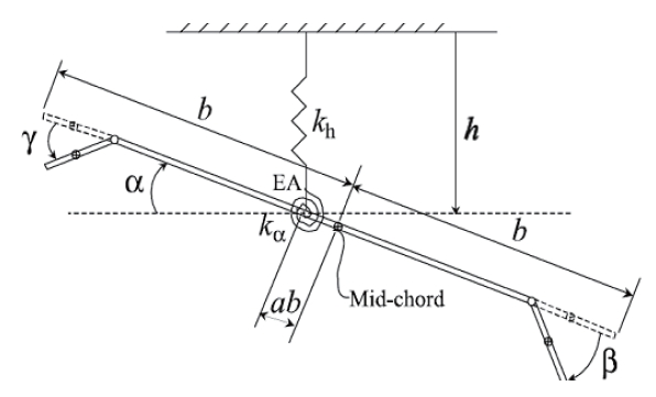
A 2-DOF pitch-plunge wing section based on previous models with both LECS and TECS is presented in Fig. 1. The system dynamics is given as follows

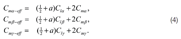
In Eq. (1), the quasi-steady lift L(h˙, α?, α, β, γ) and aerodynamic moment M(h˙, α?, α, β, γ) are defined as


where
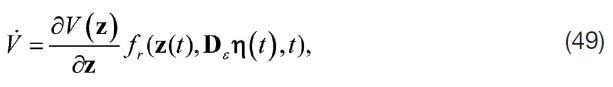
The governing equation can be written into the inputoutput representation using Eqs. (2) and (3). Motivated by Chen et al. (2008) and Zhang et al. (2005), this representation will facilitate the ensuing robust adaptive feedback control design

where x = [α,
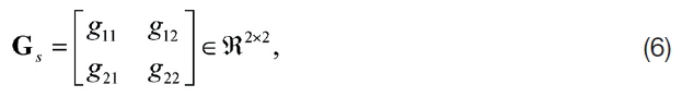
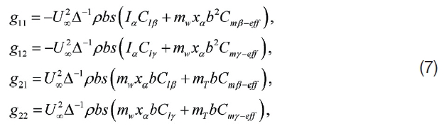
where the constant matrix entries g-
where Δ = det(Gs) =
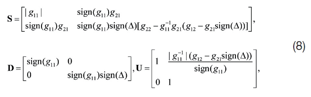
where the notation sign(*) represents the standard signum function. In this paper, the signs of the leading principal minors of the input gain matrix G-s are assumed to be known for purposes of control design, which implies that the diagonal matrix D is known. After applying the matrix decomposition property and multiplying both sides of Eq.(5) with M = S?1 ∈ R2×2, Eq. (5) can be rewritten as

where M is a symmetric, positive definite matrix and f(x, x˙ ,θ1) = M?h(x, x˙ , θ2) ∈ R2 contains parametric nonlinearities.Note that M is assumed to be bounded by
where m, m ∈ R are the minimum and maximum eigenvalues of the matrix M. The tracking error e1(t) ∈ R2 for the aeroelastic system can be defined as e1 = Xd ? X, where the desired output vector


Then, based on the above error system definitions, a composite error signal z(t) can be defined as follows
After taking the time derivative of r and substituting the derivative of e2, the following equation can be obtained as follows

After multiplying both sides of Eq. (14) by M and applying the definitions given in Eqs. (9) and (12), Eq. (14) can be rewritten as

Furthermore, given a strictly upper triangular matrix U=DU?D, the open-loop dynamics of Eq. (15) can be rewritten as follows

while above equation can be further rewritten as

where the linear parameterization term Y(x¨d, x˙ , x, e˙ 1, e1, u) θ ∈ R2 is defined as follows

3. State Feedback Control Development
In this section, all state variables in Eq. (1) are assumed to be available for measurement. To facilitate the ensuing control design, the following auxiliary control matrix is given as

where Y

where K, k
where the constant adaptation gain matrix Γ ∈

Note that the strict triangular structure of U in Eq. (18)implies that u1 only depends on u2 but u2 can be determined independently of other control inputs since the diagonal elements in U are all zero. Thus, the control law can be implemented by designing u-2 first, then using that design in the computation of u-1. After substituting Eq. (20) into the open-loop dynamics given in Eq. (17), and then multiplying both sides by M, the following closed-loop system dynamics can be obtained

where θ?(
In this section, a non-negative Lyapunov candidate function V(t, z) ∈
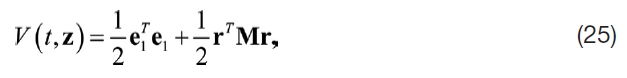
which can be upper and lower bounded as
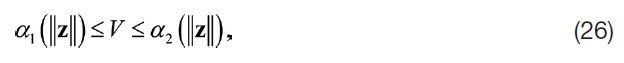
where α1('z'') and α2('z'') are class K∞4 functions given as
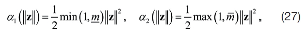
where the assumption stated in Eq. (10) has been utilized. After taking the time derivative of Eq. (25), and then substituting Eqs. (12) and (23), the following result for V(
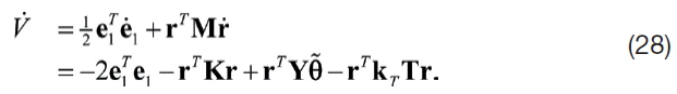
By applying the expressions given in Eq. (19), the expression in Eq. (28) can be rewritten as follows
where
Then, V˙ (
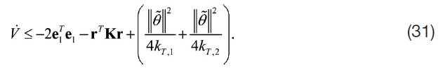
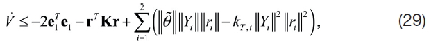
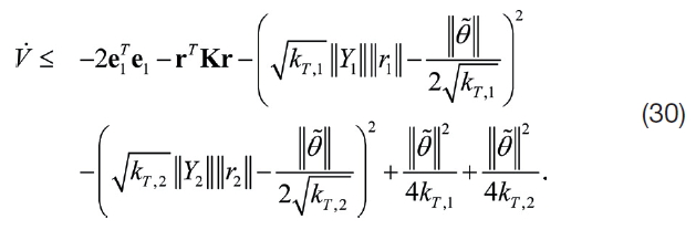
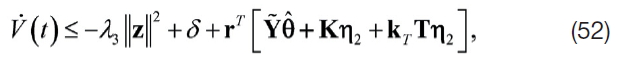
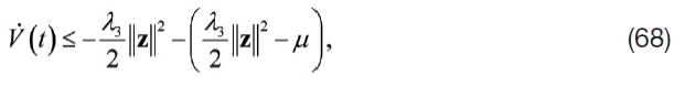
According to the definition of z(t) given in Eq. (13), the upperbound for V˙ (
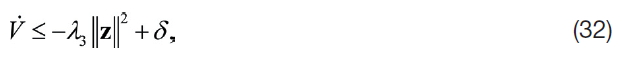
where λ3 = min{2, λmin(K)} while λmin(K) represents the minimum eigenvalue of K. The constant δ is given by
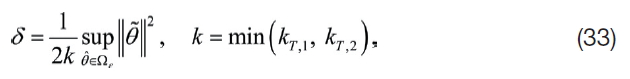
where the supremum exists since parameter projection operator defined in Eq. (21) ensures the boundedness of the parameter estimates, which implies that the parameter estimates error is also bounded. From Eq. (32), it is also easy to show that

where
while γ('z'') is a positive-definite function.From the results in Eqs. (27) and (34), all conditions for the following theorem (Khalil, 1996) are satisfied.
Theorem 4.18 (Khalil, 1996): Let D ⊂
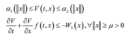
∀
μ < α2?1(α1(r))
Then, there exists a class of KL function and for every initial state
Moreover, if
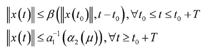
Thus, the error signal ''z'' is GUUB
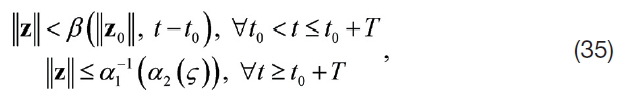
where β(·, ·) is a class KL function while T depends on ''z0''and ?. From Eq. (33), kt can be made large enough such that the upper bound for ''z'' can be made arbitrarily small.
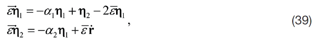
In this section, it is assumed that the only measurements available are the pitching and plunging displacements, while the remaining states can be estimated by using of HGO. An estimated composite error signal z?(
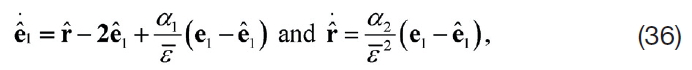
where α
η(
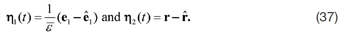
Based on Eq. (37) as well as the definitions for z? (

where Dε ∈
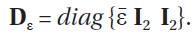
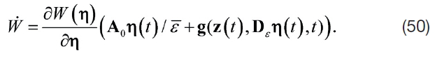
After differentiating Eq. (37) as well as taking advantage of the definition in Eq. (11), Eq. (12) and the design of Eq. (36),the following observer error dynamics can be obtained
where

where g ∈

while α
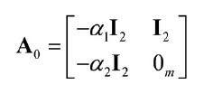
is Hurwitz. The boundary-layer system
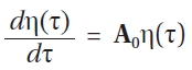
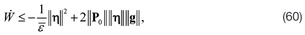
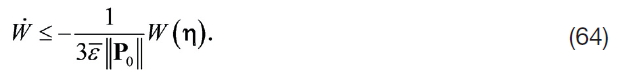
induces a Lyapunov candidate function W(η) = η
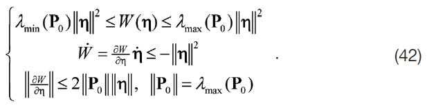
Note that in the above equation, λmax (P0) denotes the maximum eigenvalue of P-0, while P0 ∈
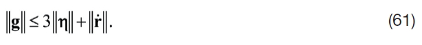
From the observer error dynamic in Eq. (39), the solution of η(
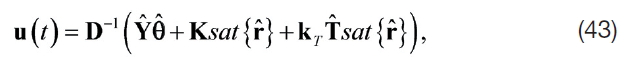
where sat{} is the standard saturation function used to limit the magnitude of the control signal to avoid the peak phenomenon. ? and T? are the regression and auxiliary matrix defined in Eqs. (18) and (19) with respect to sat {z?} instead of z(t). K, kT are defined in Eq. (20), θ? (

The saturation of input is applied outside a compact set
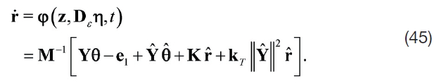
After combining Eqs. (17, 40, 41, 45), the following closedloop error dynamics are obtained
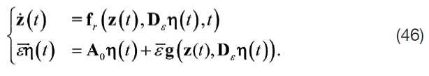
The OFB stability proof in this paper can be split into three steps in order to reduce the overall complexity. First, the existence of a positively invariant set for the solutions of Eq.(46) will be verified. Then, the boundedness of solutions of Eq. (46) is regained in the second step provided the trajectory(z(
In the ensuing stability analysis, Z is defined to be any compact set in the interior of Dz such that
Theorem 1: (Invariant Set Theorem) Given Σ =
First of all, given the following composite Lyapunov function Vc(z, η)
where V(z) and W(η) have been previously defined in Eqs. (25) and (42). Then, after taking the time derivative of Eq. (47) along the trajectory of Eq. (46), it’s straightforward to see that

where V˙ (
In this theorem, our goal is to prove that V˙ c'∂Σ ≤ 0 while the notation ∂Σ denotes the boundary of the compact set Σ.Inside the set Σ =

where Eqs. (45) and (46) were utilized in above equation.
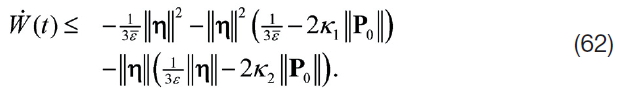
By using the results in Eqs. (28) and (32), Eq. (51) can be rewritten as follows
where ?(

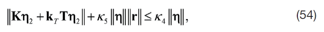
where k4, k5 ∈

From Eq. (42), it is straightforward to see that ''η(
Therefore, Eq. (55) can be rewritten as follows

From Eq. (26), any c > 2λ2δ/λ3 and z(
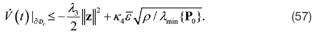
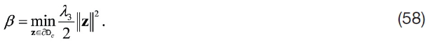
Motivated by Eq. (57), ε1 can be defined as
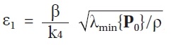
, where β ∈ R is defined as follows
Then ∀0 < ε? < ε1 and η(

Next, ?(.) of Eq. (50) can be upperbounded as follows
where P0A0 + A0 TP0 = ?I4. By using Eq. (41) and the fact that ε? is strictly less than 1, the following inequality can be obtained
Note that z(
According to Eq. (42),
Then, given a choice of
a choice of ρ= 36k2 2 ''P0''3 ensures the following result
∀0 < ε? < ε2. Finally, by defining ε?1 = min{1, ε2, ε3}, Eq. (63)implies that Σ =
Theorem 2: (Boundedness Theorem) There exists an ε?2 ≤ε?1 such that ∀ε? ∈ (0, ε?2], any trajectory (z(t), η(
By using the boundedness of z(0) and z?(0), the definition of Eq. (37) implies that
is a positive constant. From the boundedness assertion on φ(z(t), η(t)),in Eq. (45) in the set
where k3 > 0 is a positive constant. Thus, the existence of a time T-c is shown to be independent of ε? such that z(
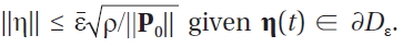
which implies ''η'' ≥ε?k2''P0''. Based on Eq. (63), W˙ (η) can be upperbounded as
By solving the above differential inequality, an upperbound for W(η(

where
Based on Eq. (42) and
Eq.(65) can be rewritten as follows
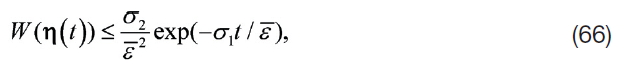
where σ2 = k6 2''P0''. Based on Eq. (66), 0 < ε?1 < ε?2 can become small enough so that W(η(
Since η(
Theorem 3: (Ultimately Boundedness Theorem) Given any solution (z(t), η(
there exists an 0 < ε?3(δ?) < ε?2 and T(δ?) > 0 such that''z(
Based on Eq. (66),
Thus, for any given small value δ?, it’s clearly to see that ε3 = ε3 (δ?) ≤ ε?2 such that ∀ε? ∈ (0, ε?3], the following upperbound can be defined
Inside the invariant set Σ, Eq. (56) can be utilized to obtain the following conclusion
where μ ∈ R is defined as follows
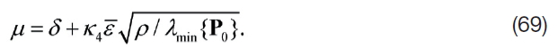
Given a compact set
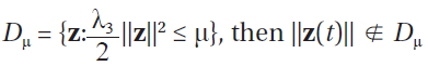
implies that V˙ (
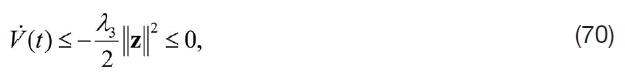
which implies that V is decreasing outside Dμ. Define Dv= {V(z) ≤ c0(ε?) =
clearly, Dμ ⊂ Dv since c0(ε?) is defined to be a non-decreasing scalar function. By choosing ε4 = ε4 (δ?) ≤ ε?2 small enough such that the set
Thus (z(
5.1 Model and control parameters
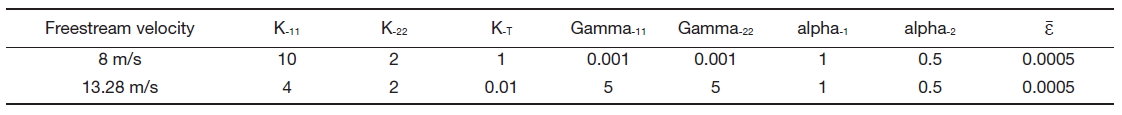
The simulation results are presented in the following paragraphs for a nonlinear 2-DOF aeroelastic system controlled by TECS and LECS. The nonlinear wing section model was simulated using the dynamics of Eqs. (1-3). The model parameters utilized in the simulation were the same as used by Platanitis and Strganac (2004) and are listed in Table 1.
The desired trajectory variables xd xd and x˙ d were simply selected as zero. The initial conditions for pitch angle α(t)and plunge displacement
The magnitude of both the leading edge β(t) and trailing edge
[Table 1.] Wing section parameters
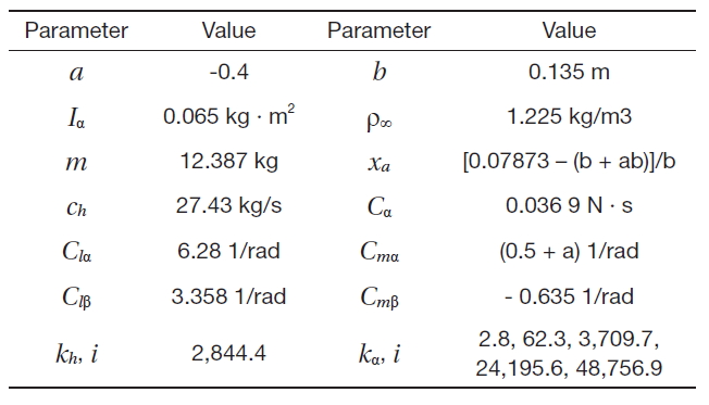
Wing section parameters
[Table 2.] Simulation parameters

Simulation parameters
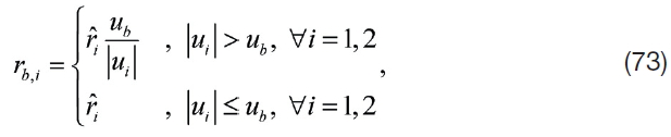
where rb denotes the limited filtered error and is used in the parameter update law Eq. (21) while u, designed in Eq. (43), denotes the actual control signal for the actuator with saturation bound
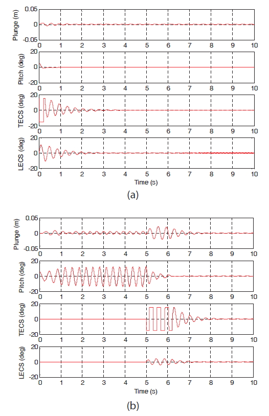
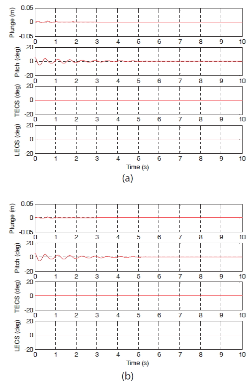
The open-loop response of the system at pre-flutter speed U∞ = 8m/s < UF = 11.4 m/s and post-flutter speed U∞ = 13.28m/s> UF = 11.4 m/s is given in Fig. .2 From Fig. 3,the convergence of the error to the origin under the proposed robust adaptive method is shown. During the pre-flutter speed, the proposed method exhibited faster settling times while the limit cycle oscillations (LCOs) at the post-flutter speed regimes were totally suppressed. In Fig.3 b, the system was allowed to evolve uncontrolled to produce LCOs due to the nonlinear pitch stiffness. The control was turned on at t = 5 s.
A robust adaptive OFB controller was proposed to suppress parametrically uncertain aeroelastic vibrations on the wing section model. The control strategy was implemented via leading (γ) and trailing (β)-edge control surfaces. The system structure and parameters, with the exception of the signs of the principal minors of the input matrix, were assumed to be unknown in the control design. By using a Lyapunov based method for design and analysis, GUUB results were obtained on the two-axis vibration errors. HGO was used to design OFB control when only the output displacements were measurable. Future work will include the experimental evaluation of the robust adaptive controller in the windtunnel laboratory at Clarkson University.