Autonomous rendezvous and docking of vehicles are essential for future space exploration of the Moon, Mars, and beyond, and for the supply and repair of vehicles such as the International Space Station (ISS). Spacecraft rendezvous and docking dates back to the manned US Gemini and Apollo programs and the unmanned Russian Cosmos missions of the late 1960s. In all the US missions, the human pilots were in the vehicle control loop during rendezvous and docking,whereas the Russians used a primarily automated approach,giving the pilots a supervisory role. The Gemini and Apollo programs developed the initial concept for rendezvous and capture. The Shuttle has demonstrated that these can be performed for various low Earth orbit (LEO) missions.Recent programs, such as Demonstration of Autonomous Rendezvous Technology (DART) (Rumford, 2002; Zimpfer et al., 2005), XSS-11 (Zimpfer et al., 2005), Orbital Express(Zimpfer et al., 2005), Automatic Transfer Vehicle (ATV)(Gonnaud and Pascal, 1999; Zimpfer et al., 2005), H-2 Transfer Vehicle (HTV) (Zimpfer et al., 2005), and the Hubble Robotic Servicing and Deorbit Mission (HRSDM)(Zimpfer et al., 2005), have been proposed and developed to demonstrate many of the technologies required for exploration that entails rendezvous and docking. Such programs have spurred significant developments in the area of autonomous rendezvous and capture (AR&C). However,the DART mission in 2005 experienced some failures.A 2006 National Aeronautics and Space Administration(NASA) report (NASA, 2006) provides an overview of the DART mishap investigation. The lessons learned from the mishap will hopefully facilitate the future development of autonomous capabilities.
Proximity operations and docking are critical phases of a rendezvous mission because highly precise translational and rotational maneuvers are required. AR&C capabilities will continue to be important for the successful execution of the various phases of a typical rendezvous mission, including the homing phase, the closing phase, proximity operations,and the final translational approach. The last two phases are critical from the perspective of mission completion and safety (Wertz and Bell, 2003). These phases are characterized by a chaser undergoing controlled motion that tracks a predetermined reference trajectory toward the docking port of the target. Like proximity operations, docking maneuvers have been accomplished in manned missions since the early days of the space program. Autonomous proximity operations are required for many future missions; however,further research and development is necessary if they are to be accomplished routinely. These requirements have led to the development and evaluation of several relative navigation sensors, such as the video guidance sensor (VGS),the global positioning system (GPS), light detection and ranging (LiDars) sensors, the laser dynamics range imager(LDRI), optical sensors, star trackers, inertial navigation systems (INS), and others. Any of these sensors can provide the basis for accurate relative positions and attitudes.Various navigation sensors are used to estimate the relative state information for feedback to an automated rendezvous and docking operations controller. Of course, autonomous spacecraft rendezvous and docking requires highly precise translational and rotational maneuvers that are integrated with precise sensors.
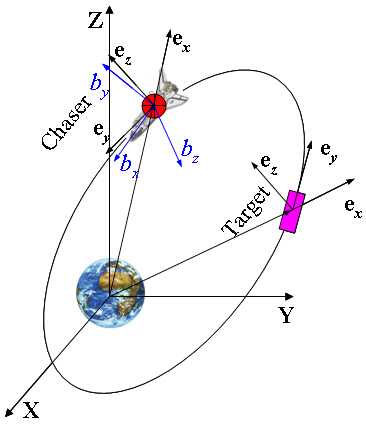
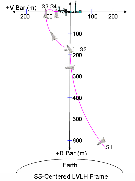
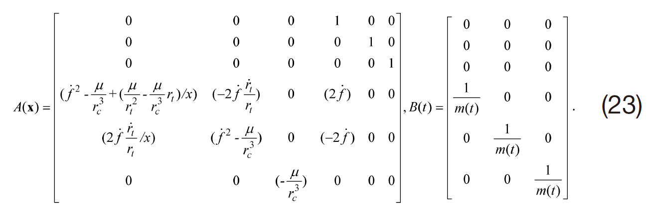
The motion of the chaser with respect to the target spacecraft is modeled by nonlinear relative equations of motion including the oblateness and aerodynamic drag.The attitude dynamics are modeled by the well-known Euler rotational equations of motion, including the gravitygradient torque and attitude kinematic equations using quaternions. Optimal control techniques are applied to the Shuttle orbiter’s manual phase flight segment covering proximity operations and docking, as shown in Fig. 1. The Shuttle program is scheduled to be retired by 2010; however,the Shuttle orbiter’s standard ISS approach technique may be extended or applied to other programs. The intent here is to develop suitable control algorithms that can facilitate autonomous proximity operations and docking. The trajectory profile design in the manual flight phase of the Shuttle is highly dependent on the payload configuration (Olszewski,1990). Payload attitude control and susceptibility to plume impingement are primary drivers in the final approach. The preferred technique for preventing plume impingement is the use of the V-bar guidance method during the final approach (Pearson, 1989), which guides the approach of the Space Shuttle along a velocity vector toward a target such as the ISS. This well-known approach is a form of pursuit guidance, and has been thoroughly investigated dating back to the Gemini program (Pearson, 1989). To initiate the V-bar approach, the active vehicle nulls the orthogonal relative velocities along the V-bar direction and accelerates to the desired closing rate along the V-bar direction, which is now along the line of sight to the target. The V-bar final approach is desirable because it is relatively fuel efficient. In addition, the constant orientation of the earth’s horizon provides a good reference for piloting, and closing rates can be easily and immediately nulled with subsequent station-keeping should some Shuttle or payload system anomaly occur (Pearson,1989). The trajectory of the Shuttle to the ISS in use since the STS-102 mission in 2001 is by default the starting point for the design of the lower surface-inspection maneuver. Figure 1 illustrates the following approach trajectory in the rotating local vertical local horizontal (LVLH) frame, centered at the ISS center of mass.
This trajectory satisfies the many constraints on visual and sensor visibility, plume impingement pressures and contamination, propellant consumption, and other factors(Cloutier, 1997). The reaction control system (RCS) of the Shuttle orbiter is used to provide thrusters for this approach trajectory. The 38 Primary Reaction Control System (PRCS)thrusters are arrayed around the Shuttle orbiter. The final orbit of the Shuttle orbiter’s rendezvous profile targets a point 183 m (600 ft) below the ISS along the R-bar direction. The Shuttle orbiter crew begins manual trajectory control at a distance of 610 m (2000 ft). The negative R-bar direction control is activated at 305 m (100 ft) to provide plume protection by inhibiting thrusters that fire toward the ISS. At the 183 m (600 ft) point, the Shuttle orbiter begins an 11.5 minute positive pitch automatic maneuver to the final ISS approach attitude.A simultaneous, manual V-bar translation of 0.3 m/s (1 ft/s)accomplishes a slow transition from the 183 m (600 ft) R-bar departure point to a final approach corridor along the ISS V-bar. In the LVLH frame, this transition appears as a gradual spiral from 183 m (600 ft) along the R-bar to approximately 350 ft (107 m) along the V-bar. From the arrival point along the V-bar, the Shuttle orbiter slowly approaches the docking port at a rate of 0.06 to 0.03 m/sec (0.2 to 0.1 ft/sec).
To effect translational control, the state-dependent Riccati equation (SDRE) (Cimen, 2008; Cloutier, 1997; Stansbery and Cloutier, 2000; Sznaier and Suarez, 2001) control and linear quadratic tracking (LQT) (Alba-Flores and Barbieri,2006; Budiyono and Wibowo, 2007; Lewis and Syrmos,1995; Naidu, 2003) control with the free-final state are both considered, and their control results are compared and discussed. To provide attitude control, a linear quadratic Gaussian (LQG) controller is used, which is a combination of a linear quadratic regulator (LQR) (Lewis and Syrmos, 1995;Naidu, 2003) and a Kalman filter. The LQR technique is a well-known and accepted theory upon which many modern controllers are based. However, most dynamic systems requiring control are nonlinear. The SDRE method entails factorization of the nonlinear dynamics into the state vector and the product of a matrix-valued function that depends on the state itself. With this factorization, the SDRE algorithm fully captures the nonlinearities of the system, expressing the nonlinear system as a non-unique linear structure known as a state-dependent coefficient (SDC) matrix that minimizes a nonlinear performance index having a quadratic-like structure. A state-dependent Riccati equation using SDC matrices is then solved in real time to yield the suboptimal control law. The SDRE control is based on the nonlinear system whereas LQT is based on the linear system. As an alternative approach, an LQT controller with the free-final state that maintains the output as closely as possible to the desired or reference output with minimum control energy is also considered.
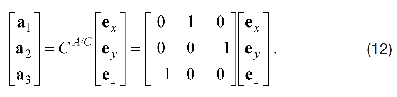
The coordinate systems used are LVLH frames centered on the target and the chaser spacecraft, and an orthogonal body-fixed frame at the center of mass and the earthcentered inertial (ECI) frame, N, as shown in Fig. .2 The LVLH frame is sometimes referred to as the CW frame (Fehse, 2003;Prussing and Conway, 1993; Schaub and Junkins, 2003), E,with the x-axis being directed radially outward along the local vertical, the y-axis along the direction of motion or velocity direction, and the z-axis normal to the reference orbit plane.In a rendezvous mission, the motion of the chaser spacecraft is commonly described relative to the target spacecraft.Instead of the CW frame E, the spacecraft local orbital frame A is adopted here to describe its motion. This frame is related to the CW frame E.
In the above, a
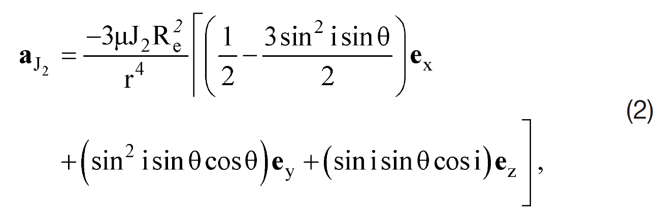
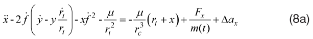
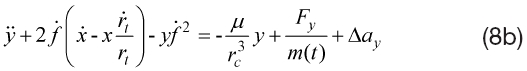
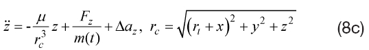
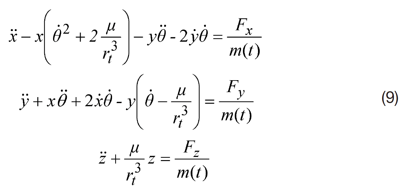
Two sets of equations of motion describing the chaser motion relative to the target in the LVLH frame are defined here. The first set includes the exact nonlinear relative equations of motion including the relative oblateness effect,J2, and the aerodynamic drag. The second set includes the linear relative equations of motions with no perturbations.The first set was used for the SDRE control formulation. The second set was used for the LQT control formulation with the free-final state. Among the many sources of perturbations,the earth’s oblateness and aerodynamic drag in the LEO are dominant. The relative effects of Earth’s oblateness and aerodynamic drag are included in the exact nonlinear relative equations for more precise dynamic modeling. In the CW frame, E, the perturbing acceleration due to oblateness is described by Prussing and Conway (1993):
where
where the subscripts,
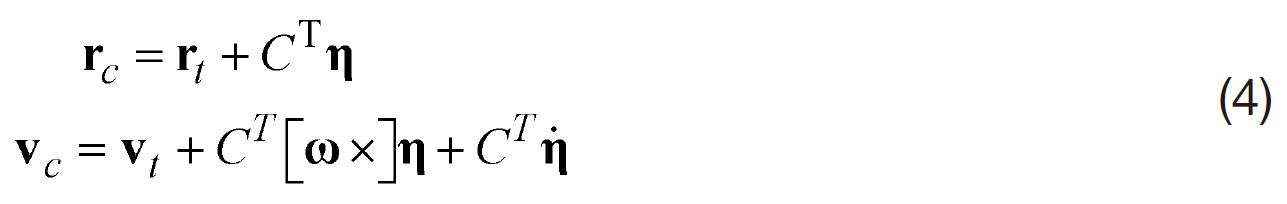
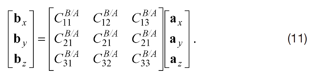
where C is the 3-1-3 rotation sequence

is the relative velocity. The ω×term is the cross product matrix. The perturbing acceleration in the CW frame due to aerodynamic drag is computed by expressing the acceleration in terms of the ECI frame(Madonna, 1997; Vallado and McClain, 2001) as
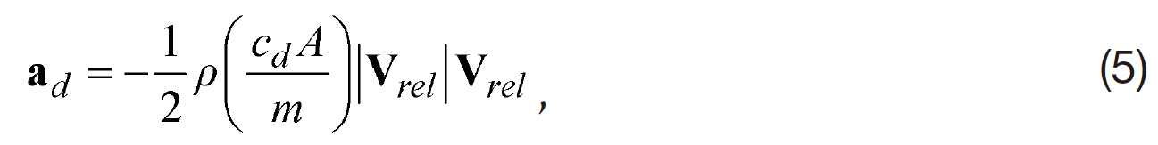
where ρ is the atmospheric density, which often is a difficult parameter to determine. The ballistic coefficient is cDA/
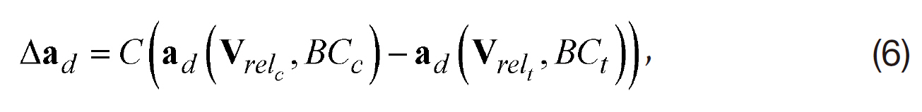
in which the drag is computed for both the chaser and the target orbit. Thus, the sum of the relative effects of Earth’s oblateness and drag becomes:

Consequently, the equations of motion for the SDRE control formulation become:
In the above,
2.3 Attitude dynamics and kinematics
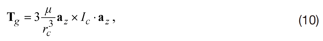
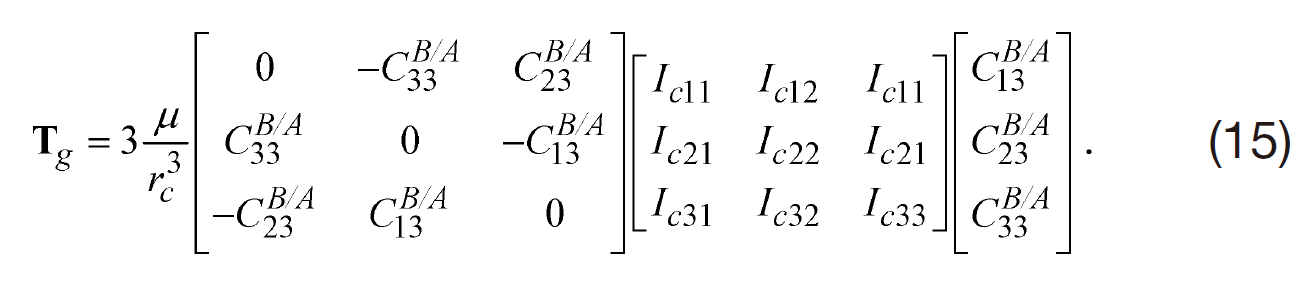
The rotational motion of the chaser expressed in the bodyfixed frame is described by the well-known Euler’s equations of motion. Like the perturbing accelerations in relative motion dynamics, the attitude dynamics also experience disturbing torques such as the torque due to aerodynamic drag, magnetic field torque, and gravity-gradient torque due to the asymmetry of the spacecraft. This study models only the gravity-gradient torque. The gravity-gradient torque due to asymmetry of the body, expressed using the local orbital frame, A, is given in vector/dyadic form as (Wie, 1998):
where
The orientation of the local orbital frame,
The direction cosine matrix, C

The angular velocity of the chaser, ω=ω


The gravity-gradient torque matrix becomes:
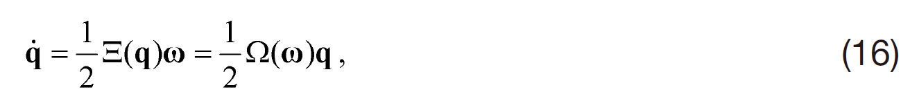
A full description of the rotational motion of a rigid spacecraft requires both kinematic and dynamic equations of motion.For most modern spacecraft applications, quaternion kinematics (Lefferts et al., 1993) are preferred. The quaternion kinematic equations are given by:
where
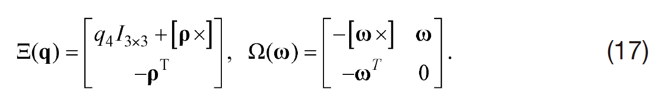
The adopted quaternion is defined by:
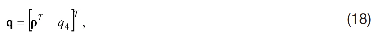
where is defined as [q1 q2 q3]T=e sin(?/2), and q4=cos(?/2),where e is the axis of rotation and ? is the angle of rotation.Euler's rotational equation of motion, including the gradient torque, is given by:
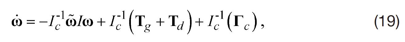
where гc is the applied control torque and where Td is the external disturbance torque, which is modeled by Gaussian-noise.
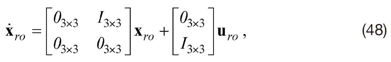
In this section, three optimal control techniques are derived for translational and rotational maneuvering. The SDRE tracking controller used with the nonlinear relative motion dynamics and the LQT controller with the free-final state used with the linearized relative dynamics are both derived for translational maneuvers. By using thrusters for translational and rotational control, both can be uncoupled to a high degree of approximation. However, a disturbance torque generated by thruster firing is considered as an unmodeled disturbance torque. The two controllers have different purposes but are executed simultaneously. The state vector for the translational maneuvers is given by:

3.1 The SDRE tracking formulation for translational maneuvers
Motivated by the LQR method, which is characterized by the solution to the algebraic Riccati equation (ARE),SDRE feedback control is an extended linearization (SDC)control method that provides an approach similar to that of a nonlinear regulation problem. For reference trajectory tracking, the regulator problem must be recast as a tracking problem. The goal is to drive the error between the reference and the output to zero with minimum control energy. The tracking problem is then formulated with the performance index as follows.
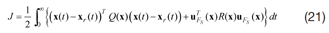


In the above, x
The SDRE method for obtaining a suboptimal locally asymptotically stabilizing solution of problem Eqs. (21, 22)is as follows.
i) Use the direct parameter method to bring the nonlinear equation into the SDC form as in Eq. (21).
ii) Solve the SDRE to obtain P(x)≥0,

Construct the following nonlinear feedback controller equation.

The resulting SDRE-controlled trajectory becomes the solution of the quasi-linear closed-loop dynamics.
Then, the state-feedback gain for minimizing Eq. (21) is:

The state weight matrix for the performance index in Eq. (21)is given by:
The control weight matrix is given by:
The weight matrices used from the initial time are readjusted at the steady-state conditions in order to reduce the steadystate tracking error The additional control forces are then generated. This tuning of the weight matrices is very important in order to generate suitable control forces with no thruster saturation. The readjusted weight matrix, Q(x),is then 1,000 times the original Q(x(
3.2 LQT formulation for relative translational motion
Tracking systems need to track a desired trajectory in some optimal sense. LQT control with the free-final state is developed to maintain the output as closely as possible to the desired output with minimum control acceleration. A linear, observable system from Eq. (9) is given as:
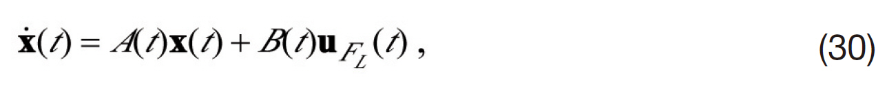
where uFL∈R3 is the control force in the CW frame from the LQT controller. The objective of the LQT controller is to control the system in Eq. (30) such that x(
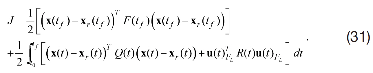
Further, the boundary conditions are defined as x(
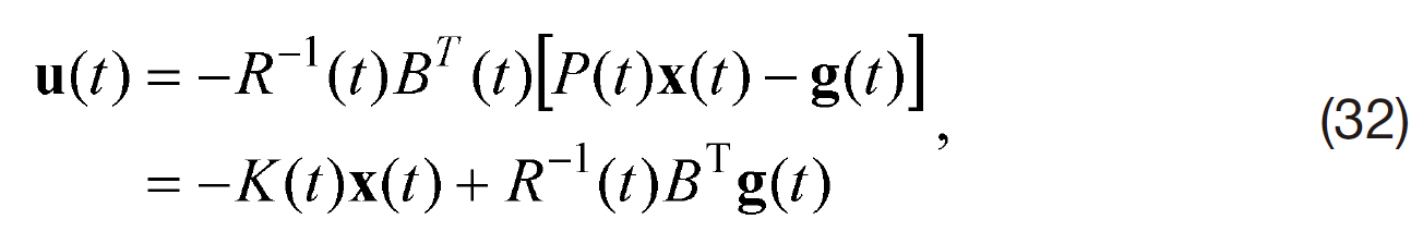
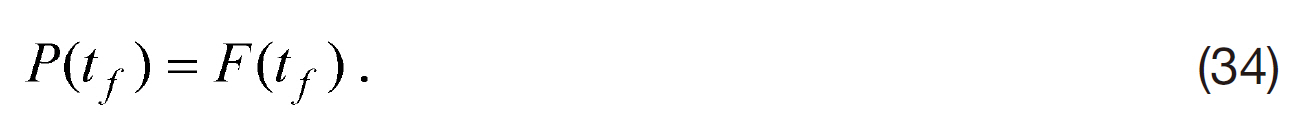
where the symmetric, positive definite matrix, P(

with the final condition being
The vector, g(

with the final condition being

Whereas the SDRE is solved online, the DRE and the nonhomogeneous vector differential equations are solved offline before control is performed. The optimal state is the solution of the linear state equation,

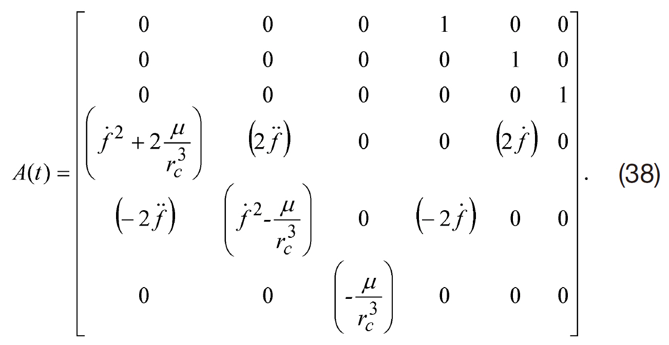
When the linearized equations of the spacecraft dynamics in Eq. (9) are adopted, the time-varying system matrix, A(
The applied weight matrices, Q(
3.3 LQG formulation for rotational maneuvers
This section describes some properties of quaternions that make it possible to realize an exact linearization of the error dynamics formulation. This study uses this linearized equation to take advantage of the simplified equation of motion to determine the precise attitude control. The control law formulation using LQR is combined with the extended Kalman filter (EKF), which leads to an LQG-type control system. The state vector for attitude control is given by:

where xa includes the quaternion and angular velocity of the chaser. The general form is given by:

where uг= гcR3 is the control torque. The goal is to drive the state to zero with minimum control energy. The regulator problem is then formulated with the performance index,
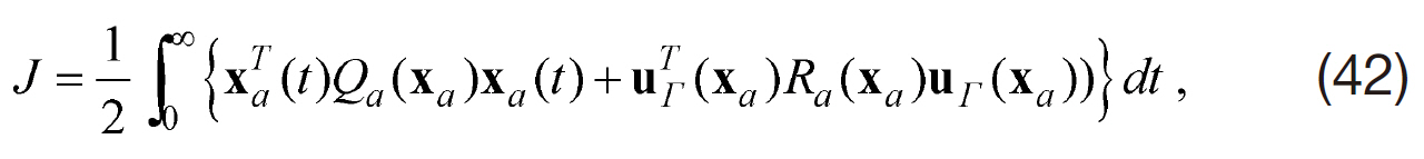
where the subscript, “a,” is used here to differentiate from translational maneuvers. The reference or desired quaternion, qd, is defined that also obeys the kinematic equation,

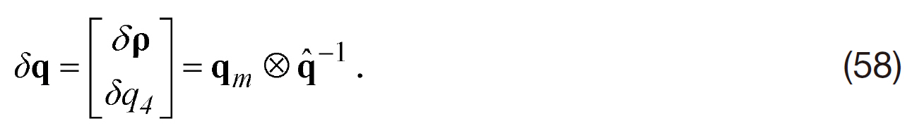
where ωd is the desired angular velocity vector and qd is assumed to be provided by on-board navigation in the target spacecraft. The error quaternion is defined as:

where ? denotes quaternion multiplication. Also, the quaternion inverse is defined by qd-1=[-ρd q4]. This work adopts the convention of Lefferts et al. (1993), who multiply the quaternions in the same order as the attitude matrix multiplication. Then, δρ and δq4 can be shown to be given by the following.


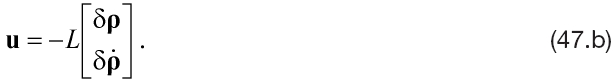
As δ

where L1 and L2 are 3×3 gain matrices. These matrices can be determined using an LQR approach starting with the following.

In the above,
where
The state weight matrix for the performance index in Eq. (42) is given by:
The control weight matrix is given by:

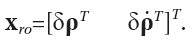
For the generation of effective control torque commands that avoid actuator saturation with good attitude tracking,the weight matrix, Qa(xa(t0)), is also readjusted at steady state as is the case with SDRE control. The ARE is solved to produce a constant gain matrix. The goal of this control is to determine a control torque, гc, in Eq. (19) that achieves the desired closed-loop dynamics given by Eq. (46). Toward this end, two time derivatives of Eq. (45a) are first taken and then substituted into Eq. (46) (Crassidis and Junkins, 2004)yielding:
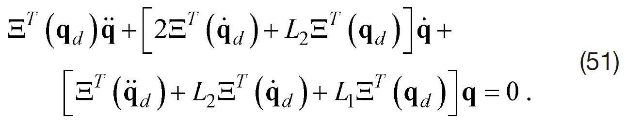
Taking the time derivative of Eq. (16) leads to:
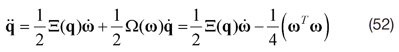
where the identity, Ω2(ω)=-(ωT ω)I4×4, is used. An identical expression for the desired quaternion is also given as:
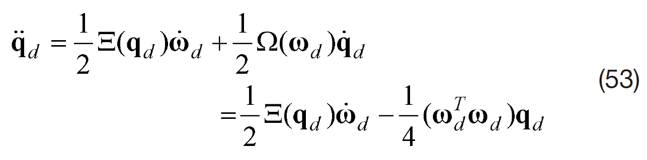
where

can be derived from Euler’s equations of motion using Eq. (19) (neglecting the unmodeled torque, Td).Substituting Eq. (16) into Eq. (52) gives:
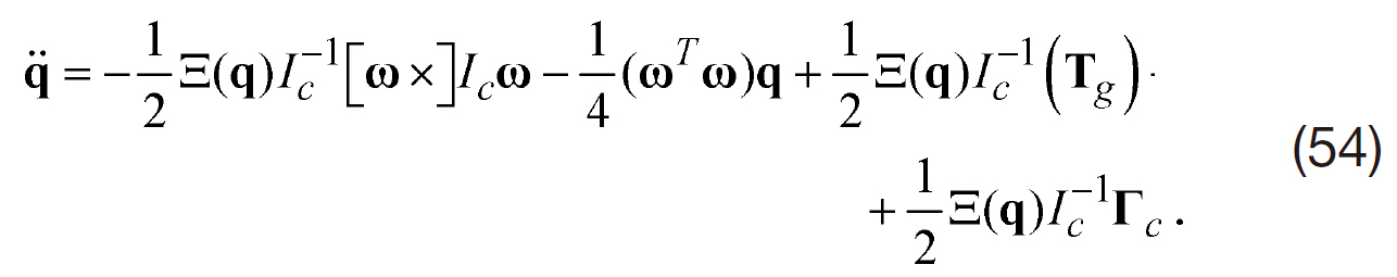
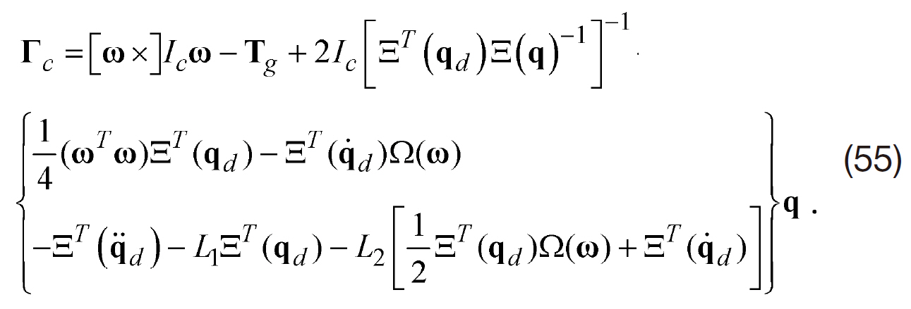
Substituting Eq. (16) and Eq. (54) into Eq. (51) and solving for гc yields:
For precision attitude control, precise attitude sensor sensors are adopted and combined with LQR control. The goal of the EKF application is the estimation of the gyro biases along all three axes and the attitude quaternions of the chaser spacecraft. The sensors used here include three axis gyros and star trackers whose output is the attitude quaternion referenced to J2000 inertial coordinates. For this sensor, a widely used model is given by the following (Crassidis and Junkins, 2004).


In the above, η

is the measured observation. A combined quaternion from two star trackers is used as the measurement. To generate synthetic measurements, the following model is used:
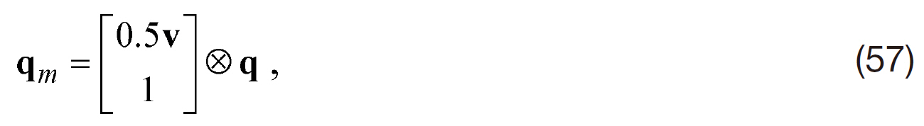
where qm is the quaternion measurement, q is the truth,and v is the measurement noise, which is assumed to be a zero-mean Gaussian noise process with a covariance of 0.001I3×3 deg2. The measured quaternion is normalized to ensure a normalized measurement. An error quaternion between the measured quaternion and the estimated quaternion of the chaser,

is used for measurement in the filter. This is computed using the error quaternion,
For small angles, the vector portion of the quaternion is approximately equal to half angles so that δ
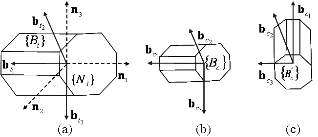
The estimated quaternions of the chaser are fed to the control torque, гc, in Eq. (54) as q. The implementation of the LQGtype control system for the chaser’s rotational maneuver is shown in Fig. 3.
4. Numerical Results and Analysis
This study tested the controllers developed here in a Shuttle-like scenario in which the proximity operations and docking have historically been performed by the crew in the manual phase flight segment, as shown in Fig. 1. A six degrees-of-freedom simulation and a passive target (ISS) were created to demonstrate the performance of the controllers. The ultimate objective was to have the chaser (Shuttle) docking port approach the target docking port leading to a soft docking with the desired attitude. There were two types of axial alignment during this phase. The first one was the simplest case in which both vehicles had the same direction of axial alignment, as illustrated by Figs. 4a and b. The second one was the case in which the chaser had to execute a pitch rotation of +90 degrees, as illustrated by Figs. 4a and c.
The quaternions of the target, q
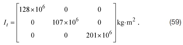
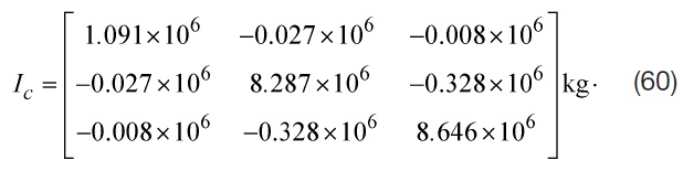
The inertia matrix of the chaser was also assumed constant and taken as follows (Nagata et al., 2001).
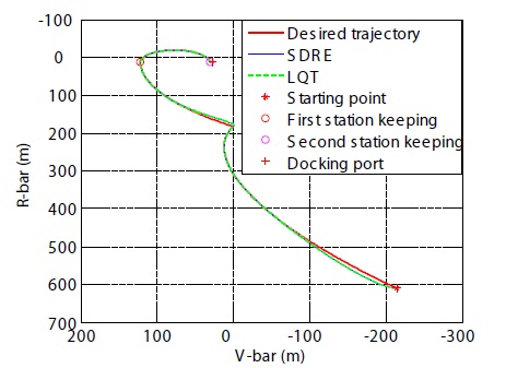
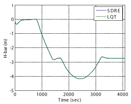
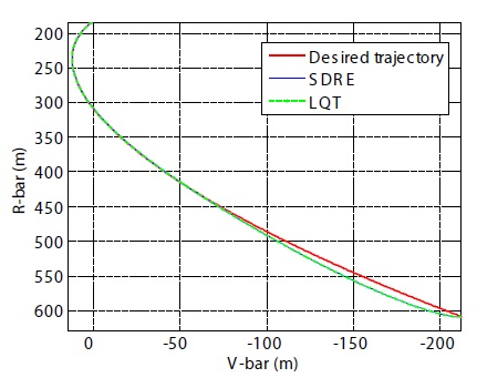
The chaser was initially located at the relative position, [609.6 213.36 0.1] m, with a relative velocity of [0.01 -0.43 0.01] m/s with respect to the target. The initial quaternion of the chaser was [0.2473 0.4123 0.8651 0.1426], which corresponded to an initial attitude of -30 degrees of pitch rotation with respect to the CW frame of the chaser. The initial biases along each gyro axis were set as 1 deg/hr (Naidu, 2003). The docking target location (Olszewski, 1990) was given as [27.30 12.71 -2.74] m in the CW frame. The flight segments were divided into a total of six stages that comprised of sub-segments. The first sub-segment started from the initial point, S1, where the final mid-course correction maneuver was executed and targeted S2, a point located 183 m along R-Bar. The second sub-segment started from S2 and continued to S3. At S2, the Shuttle started a positive pitch maneuver to the LOS of the target V-bar; the third was the first station-keeping to capture the LOS of the target; the fourth was the V-bar approach toward the target V-bar; the fifth was the second station-keeping location to decrease the approach velocity and ensure capture of the LOS; and the final sub-segment was the straight-line V-bar approach intended to accomplish soft docking. The simulation lasted for 68 minutes from the holding point, S1, to the target docking port with a step size of 0.1 seconds. Whereas the translational control was initialized at the beginning of each sub-segment, the attitude control was initialized twice to execute axial alignments. The first attitude was initialized at S1, and the second attitude was initialized at S2. Since the H-bar relative motion in this scenario was much smaller than the R-bar and V-bar relative motions, a planar motion perspective was used to better illustrate the results. The results of translational maneuvering were independently determined by both SDRE control and LQT control. The data were then plotted together from the holding point to the target docking port.
4.1 Results of translational maneuvering
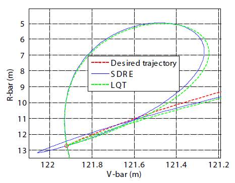
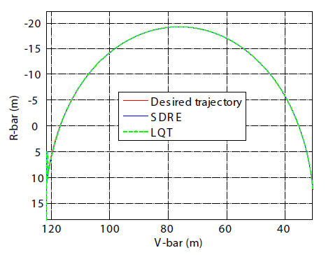
Figures 5 and 6 show proximity operation trajectories and out-of plane motions for the entire duration of simulation. Using the CW guidance scheme and final straight-line approach guidance with subcentimeter-per-second velocities, the reference trajectories were autonomously directed to the controllers. The transfer time and the nominal trajectory for the R-bar relative motion were determined by the CW terminal guidance scheme (Fehse, 2003; Prussing and Conway, 1993). Figures 7 and 8 show the fly-around maneuver from S1 to S2 for 13 minutes, and the fly-around maneuver from S2 to S3 for 10 minutes, respectively. As soon as each sub-segment was complete, the newly initialized control was applied sequentially to the next sub-segment.
After the second sub-segment was completed, a five minute period of station-keeping was executed to ensure proper LOS alignment by nullifying the arrival velocity generated by the CW terminal guidance (Fehse, 2003; Prussing and Conway, 1993), as shown in Fig. 9. After the fly-around maneuver from S2 to S3 was complete, the chaser needed to align its attitude
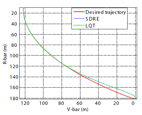
with the target LOS to the docking port during the stationkeeping period. Five minutes was considered an adequate amount of time to align with the LOS during the stationkeeping phase. Once the LOS was acquired during the station-keeping phase, the chaser prepared for the straight V-bar final approach phase and additional control forces were generated so that the chaser would not drift. After the first station-keeping period was complete, a V-bar hopping approach along the LOS was executed for 25 minutes, as shown in Fig. 10. The nominal V-bar hopping trajectory and the transfer time were also determined by the CW terminal guidance scheme, which typically provides a fuel-efficient approach.
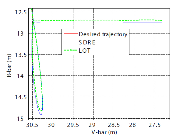
The chaser then executed a second period of stationkeeping prior to the straight LOS final approach, shown in Fig. 11, for five minutes. Unlike the first station-keeping period, the chaser’s arrival velocity was opposite to that of the arrival velocity from the second R-bar maneuver. During the second station-keeping period, the chaser slowed the arrival velocity, again aligned the LOS to the docking port,and prepared for the straight LOS final approach. After the second station-keeping phase was completed, the chaser spacecraft completed the straight-line V-bar approach to dock with the target, as shown in Fig. 12. A straight-line V-bar guidance approach with very slow constant velocity was
specified to ensure safety and avoid an unacceptably high physical impact on the target.
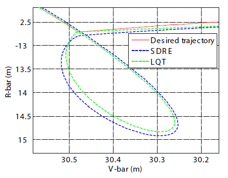
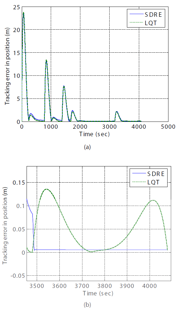
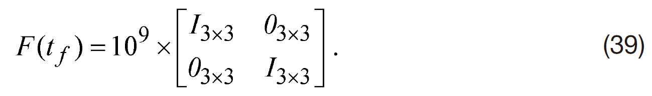
According to the docking constraints (Pearson, 1989) in use for the Shuttle and the ISS, the lateral docking tolerance is a maximum of 0.330 m (13 inches), the lateral velocity tolerance is 0.0457 m/s (0.15 ft/s), and the closing velocity tolerance is 0.0914 m/s (0.30 ft/s). It is especially important to note the position tracking error and approach range rate to monitor these conditions. In order to facilitate an effective assessment of whether or not these conditions are met, the final straight-line V-bar approach over the last 10 minutes was magnified. After control initialization in each sub-segment, the tracking error gradually decreased.This decrease in the tracking error is thus acceptable for achieving soft docking. As the translational maneuver was stabilized, the controlled state tracked the reference state more closely. The SDRE control achieved this accuracy as a result of adjusting the weight matrices in the final approach phase. However, LQT control with the free-final state could achieve very precise position tracking at the final stage by the use of a large weight-matrix, F(
position tracking error during the entire simulation. While the approach trajectory using the SDRE controller shows a constant straight-line trajectory whose error is less than 0.02 m, the one resulting from LQT control with the free-final
[Table 1] Performance in translational maneuvering in the final straight-line V-bar approach
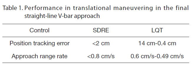
Performance in translational maneuvering in the final straight-line V-bar approach
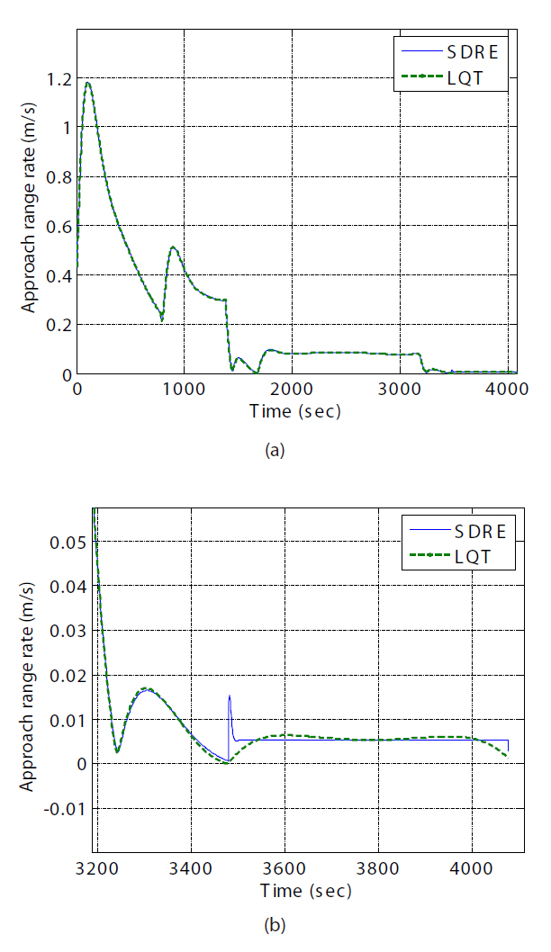
state shows a variation from about 0.14 m to 4×10⁻³ m at the final time, as shown in Fig. 13b. The approach range rate using SDRE control, shown in Fig. 14a, converged to 0.0077 m/s, whereas the approach range rate using LQT control with the free-final state, shown in Fig. 14b, dropped to 0.0049 m/s. The performance regarding translational maneuvering in the final approach is listed in Table 1.
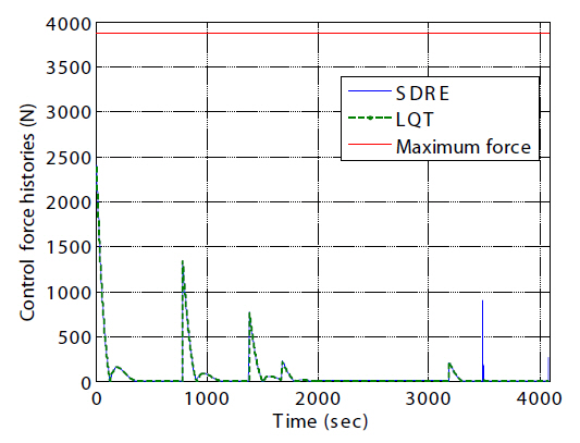
The control force histories produced by the two controllers are shown in Fig. 15. The figure also shows that the additional control forces that resulted from the readjustment
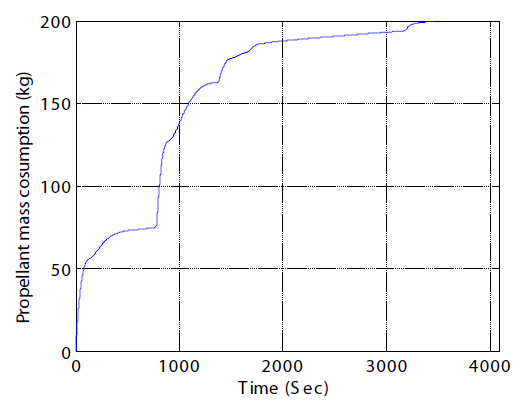
of the weight matrices in the SDRE controller increased impulsively before the final straight-line approach. LQT control with the free-final state shows that the chaser spacecraft more precisely approached each destination(shown in Fig. 1 as S2, S3, and the docking port) than the SDRE controller did. The translational maneuvers using the SDRE controller by adjusting the weight matrices in the straight-line LOS final approach could track the reference state provided by the straight-line guidance scheme and avoid thruster saturation. The tracking error was effectively reduced. However, additional control forces were required in straight-line maneuvering using the SDRE controller. Unlike LQT control with the free-final state, the effects of relative perturbations to the nonlinear system were considered in the SDRE approach in an attempt to control the translational maneuvering more precisely. For more precise translational maneuvers, the SDRE controller using nonlinear relative motion dynamics including relative perturbations can be closer to true system control than LQT control with the freefinal state. As the control forces and torques are generated,propellant mass is consumed, resulting in variations in the total mass and moment of inertia of the chaser. Figure 16 shows the propellant mass consumption as a result of the applied control forces and control torques. This study assumed that the locations of all RCSs were known so that the propellant mass consumed by the control torques could be computed. The total is the sum of the mass consumed by both the control forces and the control torques. This study
assumed that the locations of all RCSs were known so that the propellant mass consumed by the control torques could be computed. The total is the sum of the mass consumed by both the control forces and the control torques.
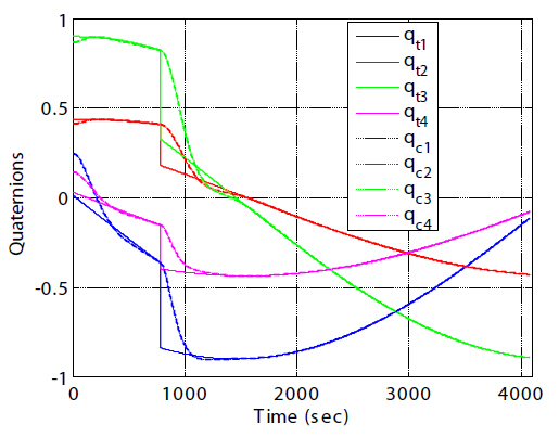
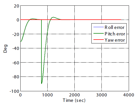
Because of varying mass, the moment of inertia is not constant. The robustness of the rotational controller was evaluated for uncertainties in the moment of inertia. The uncertainty was quantified by adding 30 percent of the initial moment of inertia to this initial value (Xin et al., 2004).Moreover, external disturbances, which were not modeled in the design of the controller, were added to the Euler rotational equation of the chaser in Eq. (19). All of the results to follow were compiled after incorporating the moment of inertia uncertainty and the external disturbances. The first rotational maneuver, illustrated by a comparison of Figs. 4a and b, was executed to align the chaser body axis with the target body axis in the first segment. The second rotational maneuver,illustrated by comparing Figs. 4a and c, was performed up to the final sub-segment after the first rotational maneuver was complete. Figure 17 shows that the chaser exhibited good attitude tracking during the entire simulation. To more clearly illustrate the geometry of the angular motion, the
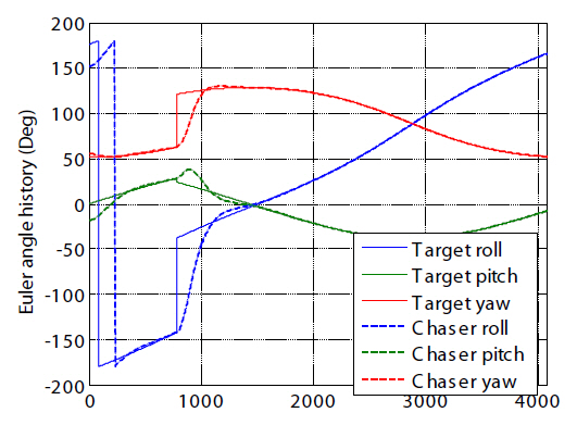
Euler angle histories of the target and the chaser expressed with the 3-2-1 rotational sequence of the chaser, as converted from quaternions, are shown in Fig. 18.
Figure 19 shows the Euler angle error history between the target and the chaser spacecraft for axial alignments that are composed of 30 and 90 degrees of pitch rotation. The target is orbiting in a near-circular 350 × 450 km altitude Earthpointing orbit. The target angular rate can then be expressed as ωt=[0
succeeded in maintaining an acceptable attitude tracking error. The rotational maneuvers thus could meet the alignment condition for the docking phase. The performance regarding rotational maneuver in the final straight-line V-bar approach is listed in Table 2.
[Table 2.] Performance regarding rotational maneuver in the finalstraight-line V-bar approach
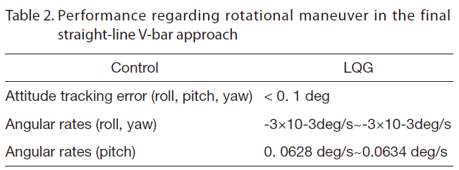
Performance regarding rotational maneuver in the finalstraight-line V-bar approach
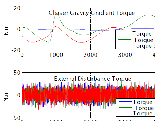
The upper plot in Fig. 21 shows the gravity-gradient torque history acting on the chaser, and the lower plot shows the external disturbance torque history acting on the chaser,which was simulated by white Gaussian-noise with mean[10 10 10]T, both of which were added to Eq. (19). Figure 22 shows the applied control torque history. Along with the two required attitude changes, the large, initial, disturbing control torques were applied and the response was then reduced to nearly zero.
This study designed a nonlinear SDRE control technique and an LQT control technique for translational maneuvers between spacecraft. The adopted SDRE control technique was designed for nonlinear relative motion dynamics, including Earth’s oblateness and aerodynamic drag perturbations.Through the SDC parameterization, a linear-like closedform structure was achieved for the nonlinear system control problem. For the tracking command, the controller was designed without increasing the state dimensions, unlike the SDRE integral servo controller formulation. The tracking results using SDRE control were successfully achieved by readjusting the weight matrices at the steady-state interval to avoid saturation. The LQT control designed for the linearized system shows that the free-final state becomes the fixed final state when the weight matrix for the final state is large. This result is very effective in meeting the required final state condition. The LQT control results can be used as a reference in designing the SDRE controller. However, for more precise control, SDRE control is preferable because the controller was designed for the nonlinear system including the relative perturbations. An LQG-type control technique was designed for the rotational maneuvers. A combination of an LQR controller and EKF estimation using star trackers and threeaxis gyros constitutes the LQG-type control technique. The weight matrices were readjusted similarly for the LQG-type control as for SDRE control to decrease the attitude tracking error to within the desired accuracy. The tracking error was maintained even in the presence of disturbance torques and uncertainties in the moments of inertia, demonstrating the robustness of this LQG-type controller. The Shuttle crew’s manual flight segment was chosen to simulate and evaluate the control techniques applied in this study. A six degrees-of freedom simulation demonstrated that the adopted control techniques can successfully conduct proximity operations and meet the conditions for the docking phase. The control techniques can also be applied to other programs that require autonomous proximity operations composed of many subphases,including docking. For executing autonomous and precise proximity operations, including successful docking,the integration of these controllers with accurate state estimation using high-precision sensors is needed.

![Standard International Space Station (ISS) approach (adaptedfrom Walker et al. [2005]).](http://oak.go.kr/repository/journal/10536/HGJHC0_2010_v11n3_206_f001.jpg)