The attitude, velocity, and position states of an inertial navigation system (INS) are obtained by integration of the measurements; this integration can lead to unbounded growth in navigational errors with time if there are initial state errors. Therefore, initial alignment is significantly important to guarantee high accuracy of the navigational systems. That is, accurate information must be available before launch.The initial position and velocity can be measured by external sensors, while the initial attitude must be estimated through initial alignments. Additionally, gyro and accelerometer biases, which are other major error sources that degrade navigational performance, must be considered. The accurate estimation of gyro biases is particularly important since these biases introduce velocity and position determination errors that are proportional to ab_gt² and ab_gt³, respectively(a: acceleration, b_g: gyro bias, t: navigation time).

The initial alignment process consists of two steps, coarse and fine alignment (Britting, 1971; Savage, 2000). The purpose of coarse alignment is to provide a fairly good initial condition for the fine alignment processing. The initial alignment angles are computed by using the average measurements for a predetermined period of time. Then, the fine alignment is commenced to reduce the error angles to as close to zero as possible. At this step, the initial attitudes are estimated from the instantaneous data of accelerometers and gyros.The velocity and position errors, which are obtained from navigational calculations performed at a stationary state,also can be used. The accuracy of the initial fine alignment is directly associated with navigational performance.

Due to its importance, many studies have been performed on this topic (Ali and Jiancheng). Conventional Kalman filtering has been used most broadly. However,its low computational speed is a big obstacle to real-time implementation. To reduce the alignment time, various low error order models and decoupled models have been derived, and other estimation algorithms including those using neural networks have been proposed to improve the slow convergence rate of the azimuth error (Cheng and De Wan, 1996; Liu et al., 2008).

Furthermore, the following additional restrictions in initial alignment algorithms for space launchers make the problem more difficult.

The stationary alignment condition of fixed launch pads restricts their observability.

The algorithm must be robust enough to guarantee its stability and convergence even in a wind-induced sway environment to which launchers are subject in launch pads.

Since launch vehicles reach their target orbits with very high velocities, inaccurate azimuth angle information can induce large lateral velocity and position errors, which also appear as orbit inclination errors. This requires that azimuth angles be measured with high precision.

Their computational speed is high enough for flight software implementation.

In the case of mechanical gyros such as dynamically tuned gyros (DTGs), the run-to-run biases cannot be ignored and three-axis biases also must be estimated during the process.

Instead of using Kalman filters, a new initial fine alignment algorithm, which can satisfy these requirements,is developed here. The proposed approach is to design a simple PI feedback controller for the estimation errors as in traditional controller design problems (Franklin et al., 1991).The reference attitudes for the closed loop control system are provided by two tilt angles that can be evaluated with precise INS acceleration measurements, and the azimuth angle, which also can be measured precisely from optical alignments. The bias levels of the accelerometers of our strapdown INS are within 0.1 mg, which enable self alignments (the tilt angles can be estimated with high accuracy, i.e., within 0.006 deg). By correcting the differences between the current

attitudes obtained by integrating INS gyro measurements and the references, the initial INS attitudes and gyro biases are estimated. In the same fashion, the observable vertical accelerometer bias is also estimated. To show the superiority of the proposed algorithm, two test results are presented here. The first test is a computer simulation for the sway environment, and the second is the flight test of Naro-1,where the alignment algorithm is implemented in the INS of the second stage.

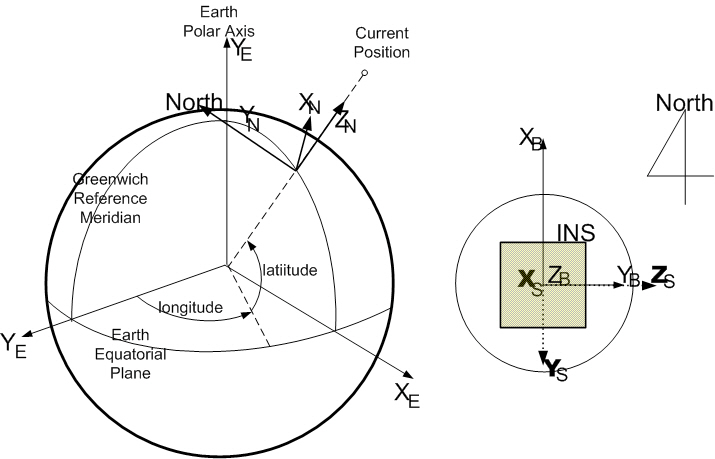
The coordinate frame for describing the algorithm is illustrated in Fig. 1. The N frame is the navigation coordinate frame for integrating the acceleration and the angular velocity, which is chosen as the north-east-down (NED)frame. The B frame is the body-fixed coordinate frame for defining the angular orientation relative to the N frame(the B frame in the stationary alignment coincides with the N frame), and the S frame is the inertial sensor coordinate frame with three axes defined by the mounting orientation of the real sensors such as gyros and accelerometers.

At the start of navigation, the INS attitude relative to the navigation frame must be available from the initial alignment process. Since the initial alignment errors due to the initial attitude errors and sensor biases are directly related to navigational performance during flight, initial alignment,which consists of analytical coarse and fine alignment, needs to be performed accurately within the given time.

In the course alignment process in this study, the tilt angles are computed as follows, using the time-averaged accelerometer measurements during the initial 30 seconds(Park et al., 1998).

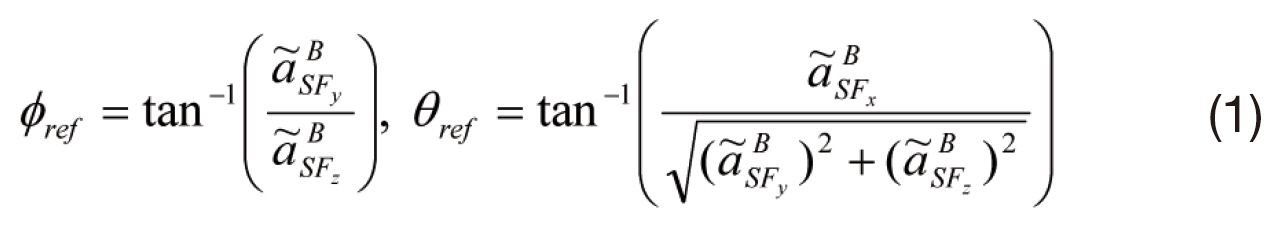
In Eq. (1),

denotes the accelerometer measurement that is represented in the B frame. If analytic coarse alignment is employed instead of optical alignment, the azimuth angle can be computed using the tilt angles and gyro outputs.

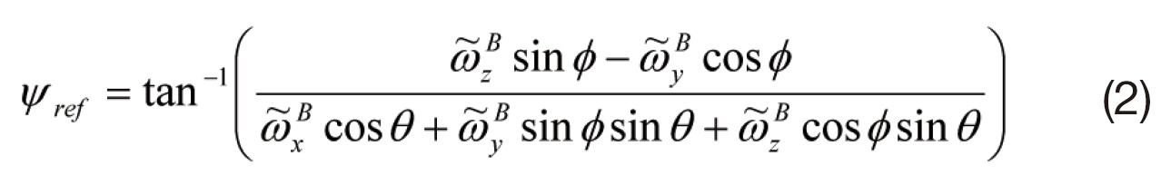
In Eq. (2),

denotes the gyro measurement that is represented in the B frame. The analytic alignment method is a rapid way of obtaining initial estimates. The bias levels of the gyros and accelerometers of our strap-down INS are within 0.2 deg/hr and 0.1 mg, respectively. Therefore, the tilt and azimuth angle estimation errors are given as follows(Park et al., 1998).

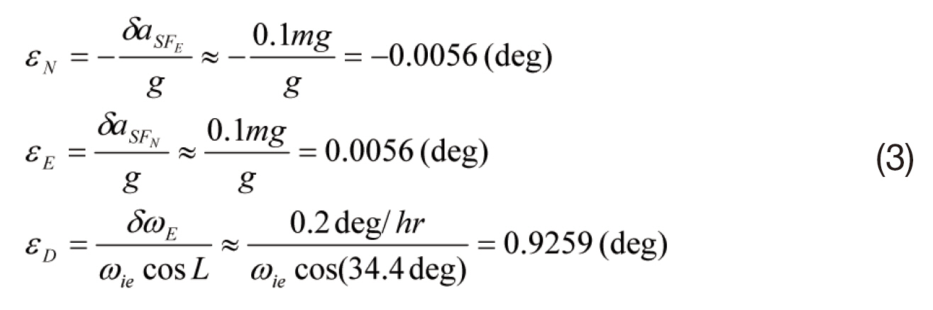
In Eq. (3), L and ω_ie denote the current latitude and earth rotational speed, respectively.

The accuracy of the accelerometers can satisfy the requirements for the initial leveling alignment within 0.014 deg while azimuth alignment, which must be less than 0.025 deg, cannot be realized with the gyros. Instead of utilizing extremely accurate gyros, optical measurements using a theodolite sighting and prism mounted on an inertial measurement unit are employed here (Cho et al., 2005).Since this technique has proven to be very accurate and readily applicable, it has been used frequently in the azimuth alignment of INS for satellite launch vehicles (Gordan, 1987;Mrus et al., 1971).

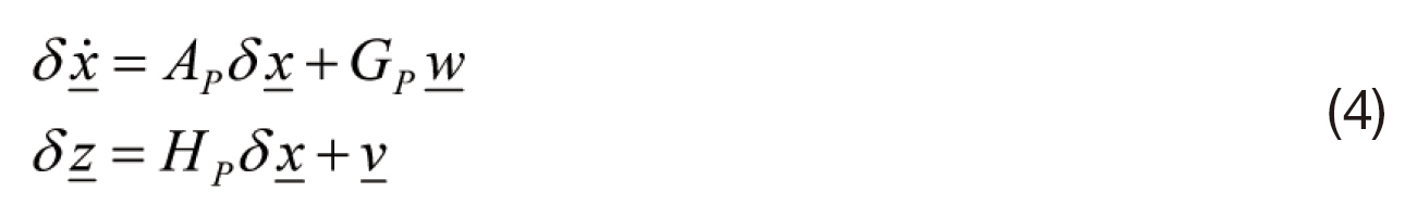
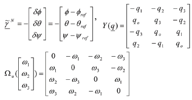
In the fine alignment of the precise alignment stage,Kalman filters are generally applied to provide estimates of the attitude errors and sensor biases. As with the design procedure of Kalman filters, a linearized error model for the inertial instrument is presented and its observability is investigated for the proposed filter. The following 10 state error models are selected since the position and velocity variations can be ignored during the alignment process that is performed before launch and the dominant error sources of the gyros and accelerometers are biases. Also, the reference frames of the error terms are chosen in such a way that the observability analysis is less complicated.

with

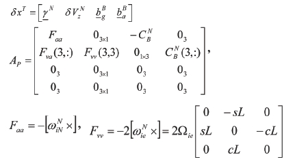
In Eq. (4), the notation is as follows.

ωCAB : Angular rate of frame B relative to frame A as projected on frame C’s axes.

CBA : Direction cosine matrix that transforms a vector from its projection in coordinate frame A to its projection in coordinate frame B.

A(i, j) : Element in the i th row and j th column of the matrix A.

A(i,:) : Vector composed of elements in the i th row of the matrix A.

γN : Attitude error defined as (γN×)=I-？NB(CNB)T.

δVzN : Z-axis velocity error in the N frame.

Here, the vertical channel is not decoupled from the horizontal channels, which is different from the error models used usually for simplified analysis of the observability of INS in ground alignment (Jiang and Lin, 1992, 1993). As in many other references, e.g., Bar-Itzhack and Berman (1988), the horizontal velocity errors can be considered as the system measurements. However, they just increase the system dimension, and they are excluded here. Instead, the INS attitudes and vertical velocity are considered as the system measurements. This means that the reference measurements are chosen as the vertical velocity and pitch and roll angles calculated by using the accelerometer outputs and the azimuth angle obtained by optical alignments.

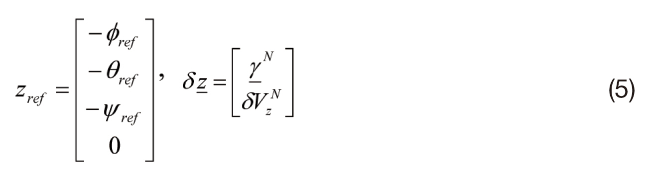
Then, the measurement matrix is given as follows.

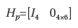
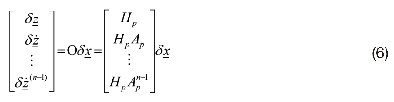
Since the error model in Eq. (4) is almost a linear timeinvariant system, its observability can be easily investigated by a rank test of the observability matrix. If the rank of the matrix is full, the system is completely observable and if not,the dimension of its null space is the number of unobservable states.

The null space of the matrix can be derived as follows. To satisfy the equations in rows 1-4, the vertical velocity and attitude error states must be zero.

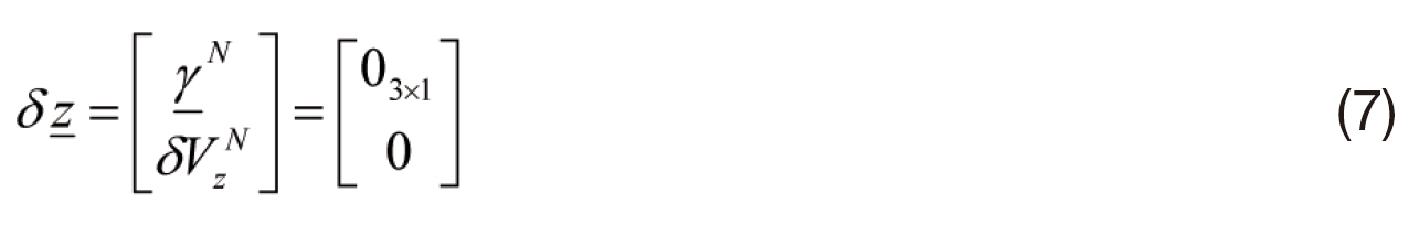
Then, to satisfy the equations in rows 5-8,

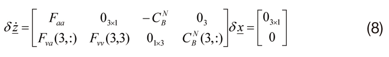
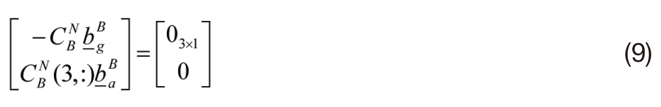
From Eqs. (7)-(9), the following relation can be derived.

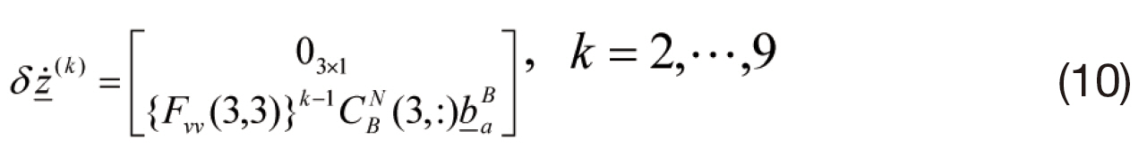
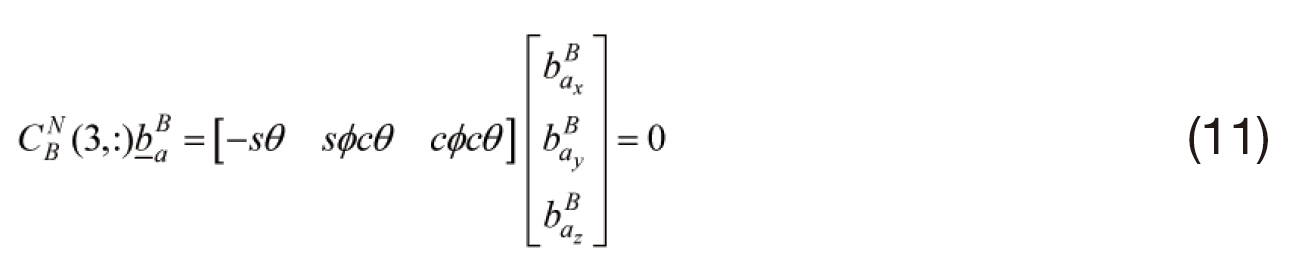
Eq. (10) shows that the dimension of the null space is two and the unobservable states are two components of

These depend on the attitude of the launcher, as shown in Eq. (11).If INS is laid horizontally, horizontal accelerometer biases are unobservable. Numerical covariance analysis for the observability problem also yields the same results although it is omitted here.

To speed up filter processing, the system is usually simplified by reducing its order and even decoupling.Instead of using these techniques, a classical controller design approach is applied here. Based on the observability of the error model, only observable states are chosen for the design of the alignment filter.

To present the concept of the proposed algorithm with the simplest example, the estimation of the attitude and gyro

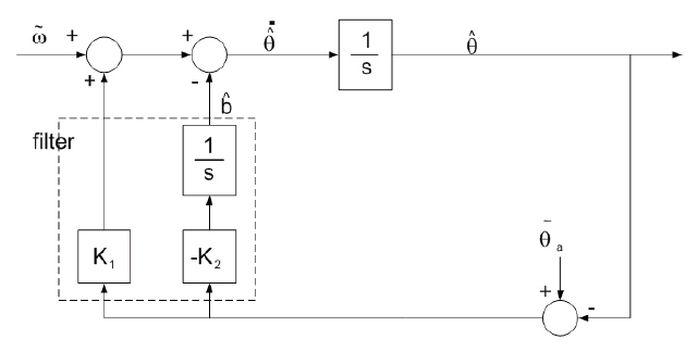
bias about a single axis is performed in this section. Then, its application to a full three-dimensional problem is described in the next section. Fig. 2 and Eq. (12) show this estimation process.

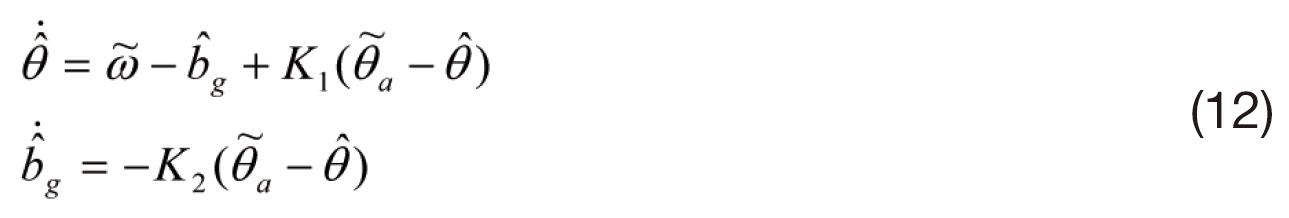
In Eq. (12), d

enotes the reference attitude obtained by the accelerometer measurement, and K₁ and K₂ are the filter gains. The feedback signal for attitude estimation is the error signal and its integral value like a proportional-integral (PI)controller. The state corresponding to the integrator is the bias. In the steady state, the error signal, i.e., the alignment error, will converge to 0, only if the filter gains are chosen appropriately by considering the closed-loop stability and filter performance. Here, the gains are determined on the basis that the settling time is about 200 seconds: K₁=0.04397 and K₂=0.00098651.

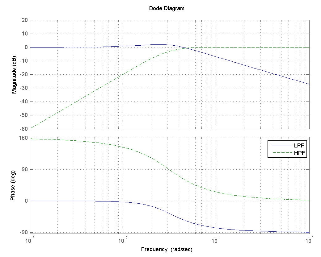
The alignment filter also can be considered as a complementary filter that blends the accelerometer output for low-frequency attitude estimation with the gyro output for high-frequency estimation, which can be seen easily from the transfer function form as follows.

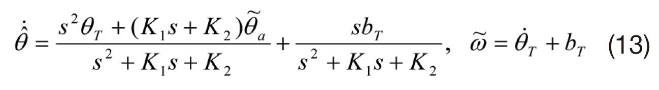
Here, the sum of the transfer functions is unity and also is the bias term filtered for estimation. Since the low-pass filter(LPF) is designed to attenuate signals with frequencies higher than 0.008 Hz, its magnitude is close to unity within its pass band, while the reverse is the case for the high-pass filter.The frequency responses of the low- and high-pass filters are presented in Fig. 3. The complementary filtering method is

commonly used for the attitude determination of unmanned aerial vehicles due to its simplicity and robustness (Euston et al., 2008).

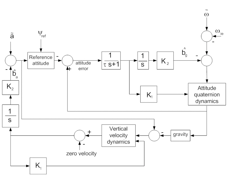
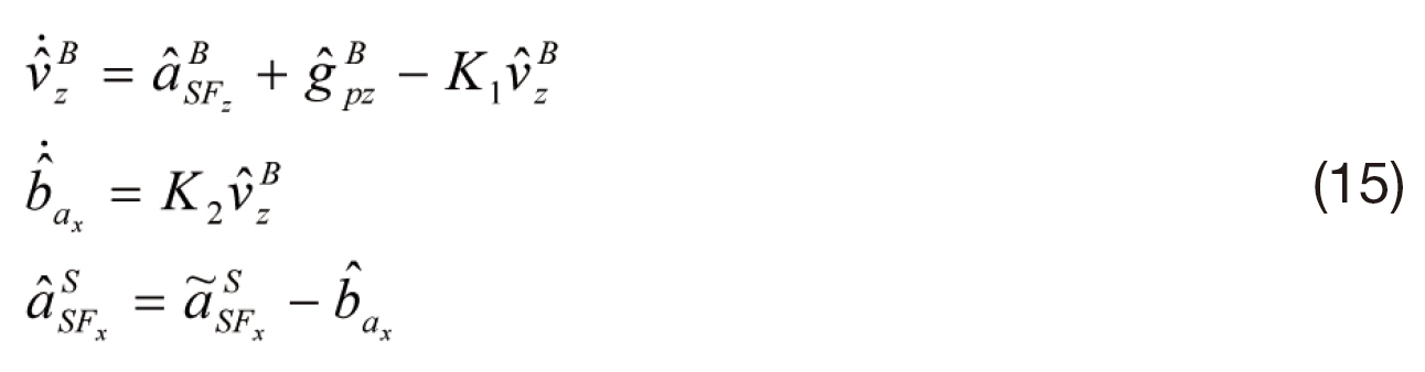
The proposed initial fine alignment algorithm is now extended to the full three-dimensional problem. From the results of observability analysis in the previous section, the unobservable horizontal components of the accelerometer biases are excluded from the estimation process. Eq. (14)represents the estimation process. The reference attitude is calculated by using the information on the tilt and azimuth angles obtained by accelerometer measurements and optical alignment, respectively. The error is then obtained by subtracting the current attitude from the reference. After filtering the error using LPF, the feedback PI controller is applied for attitude and bias estimation. Then, the attitude estimates are obtained by the integration of the gyro measurements with the error correction term. Here, the measurements are compensated using the bias estimates,which also are obtained by integration of the filtered error.The estimation loop of the accelerometer bias can be constructed in a similar way, where the error signal is the difference between the vertical accelerometer measurement and the vertical gravity component, as can be seen in Eq.(15).

Figure 4 illustrates the alignment process, which considers the full three-dimensional kinematics. In the accelerometer bias estimation, the attitude estimates are used to compute the gravity component that is projected in the vertical axis.The LPF in Fig. 2 is necessary to decrease the unwanted high-

highfrequency information from the quantization errors of the INS analog-to-frequency (AF) converter and sway disturbances.The AF converter is necessary to change the analog outputs of the gyros and accelerometers of the navigation computer to digital values. The quantization level of the gyros and accelerometers are 2 arcsec/pulse and 1.7 mm/sec/pulse,respectively, at every 0.01 seconds, which means that the rate resolution of the gyros is 0.05 deg/s and the acceleration resolution is 0.17 m/s2. Therefore, it is necessary to introduce smoothing filters to attenuate the instantaneous angular change of 0.01 deg induced by the accelerometer outputs.Here, the LPF is chosen as a first-order transfer function type.

Attitude and gyro bias estimation (Lee et al., 1997)

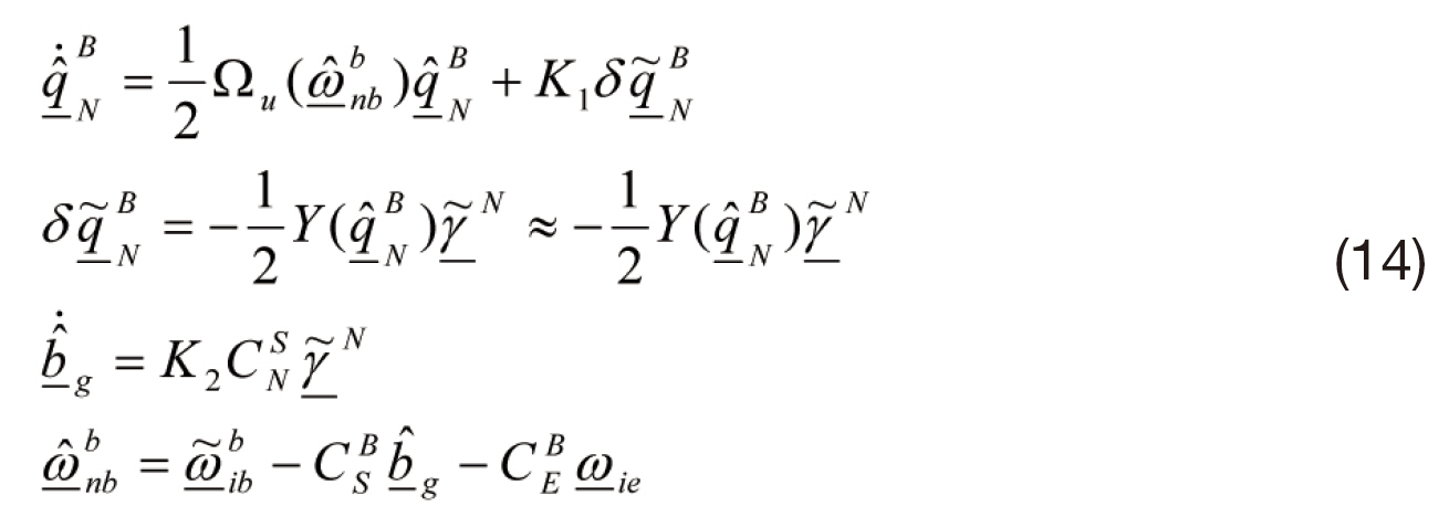
where

Vertical accelerometer bias estimation

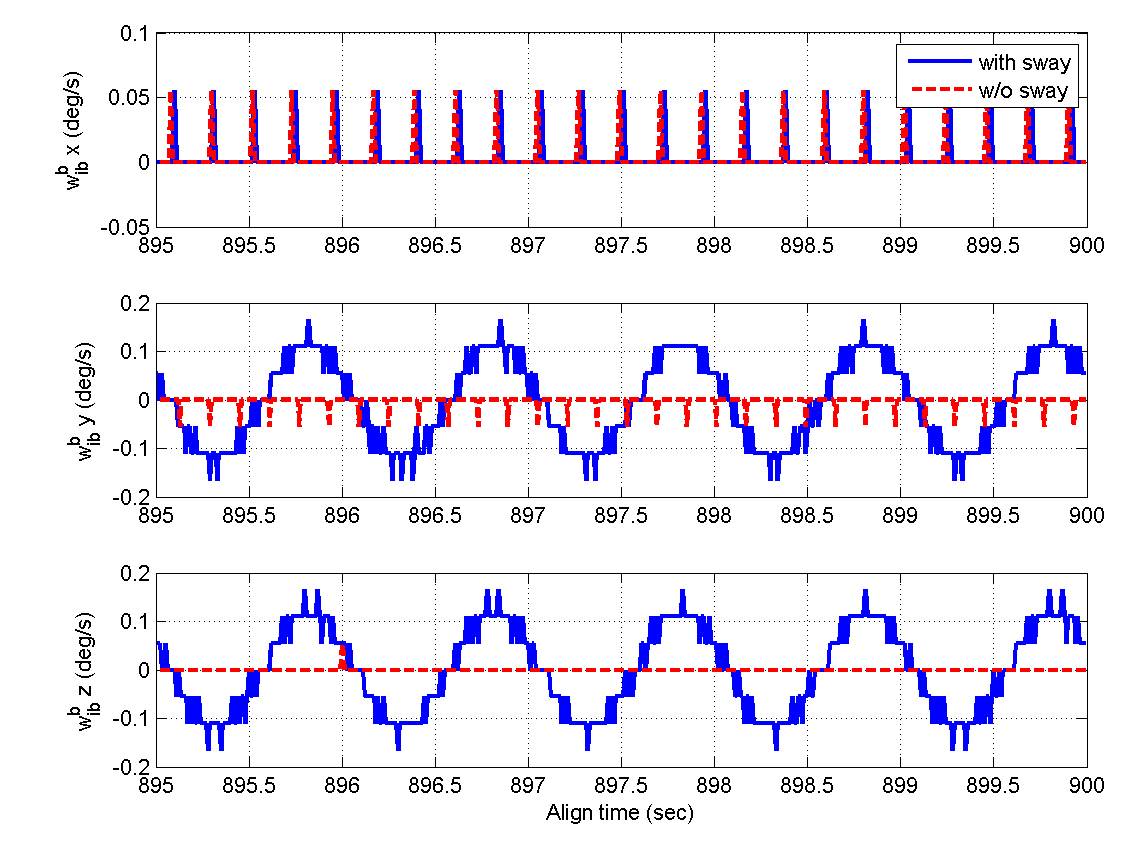
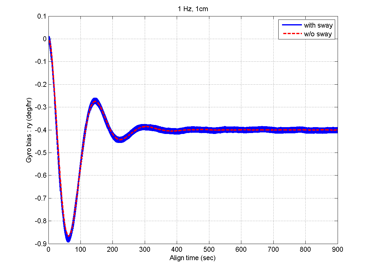
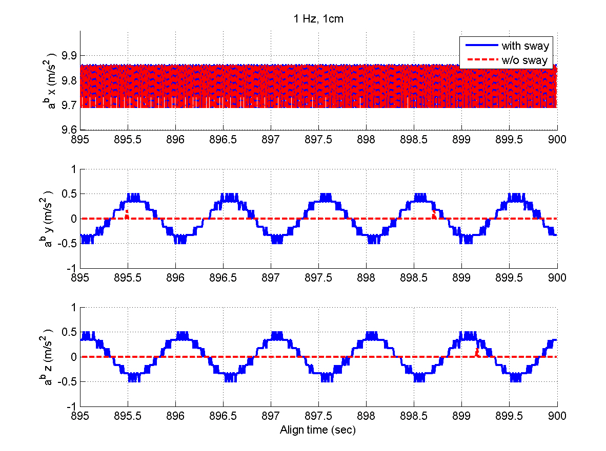
This section deals with performance evaluation of the alignment algorithm. First, the results of computer simulation are presented. Then, the flight test results are shown. In the computer simulation, the INS measurements are generated by considering the AF converter characteristics and the gyro/accelerometer biases are assumed to be the most dominant sensor errors. The simulation conditions for the windinduced sway environment are summarized as follows.

Initial attitude error (the true attitude is set to zero)

(ο/(0), θ(0), ψ(0)) = (25, 50, -40) (arcsec)

Gyro bias

=(0.2, -0.4, 0.5) (deg/hr)

Accelerometer bias

=(50, 50, 40) (μg)

Sway condition

- Maximum displacement: 1 cm

- Frequency: 1.0 Hz (sine function)

Wind direction: north and east, respectively

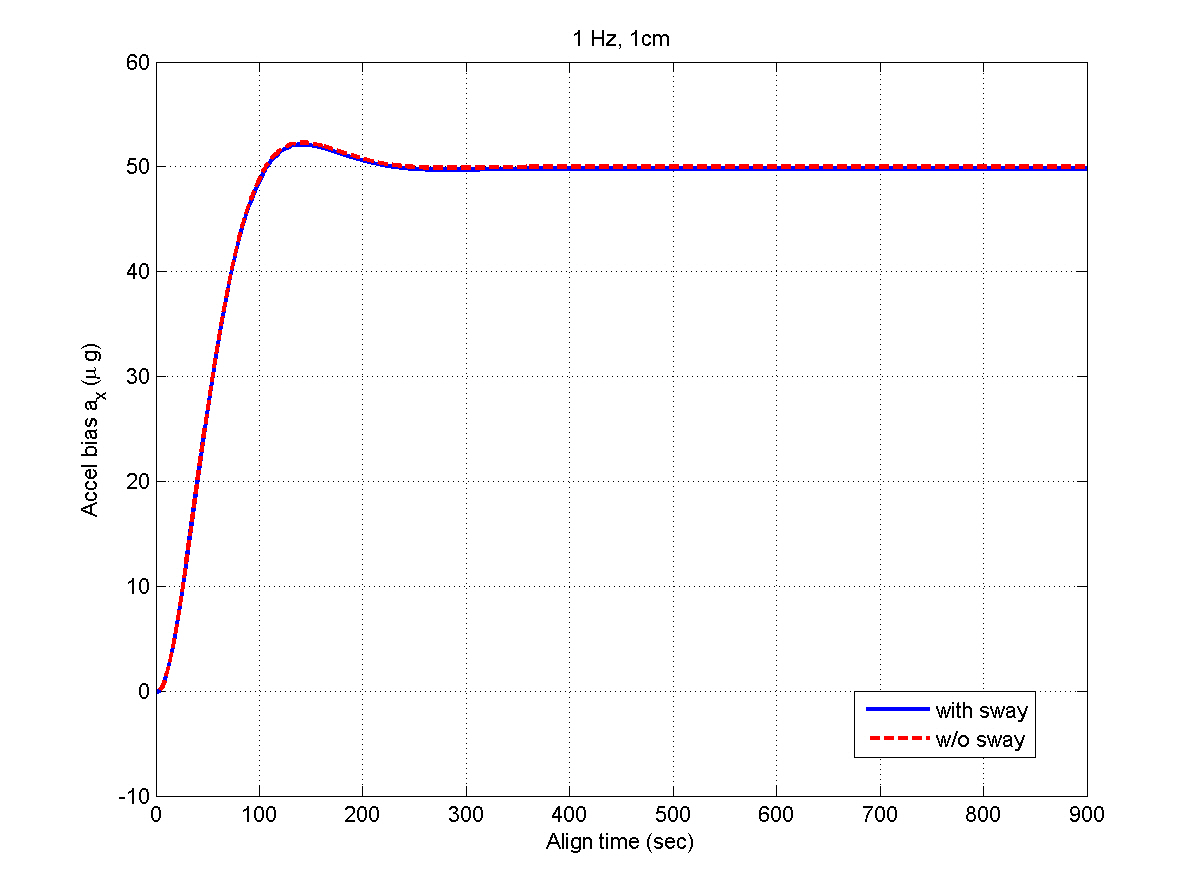
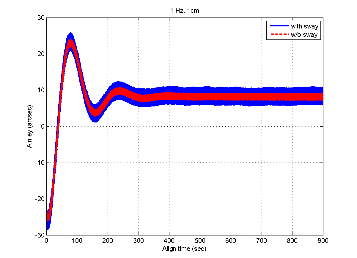
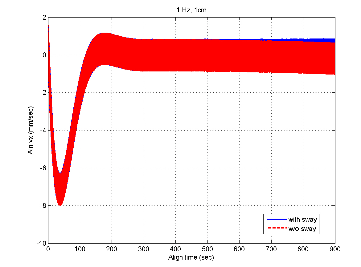
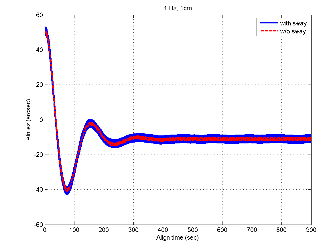
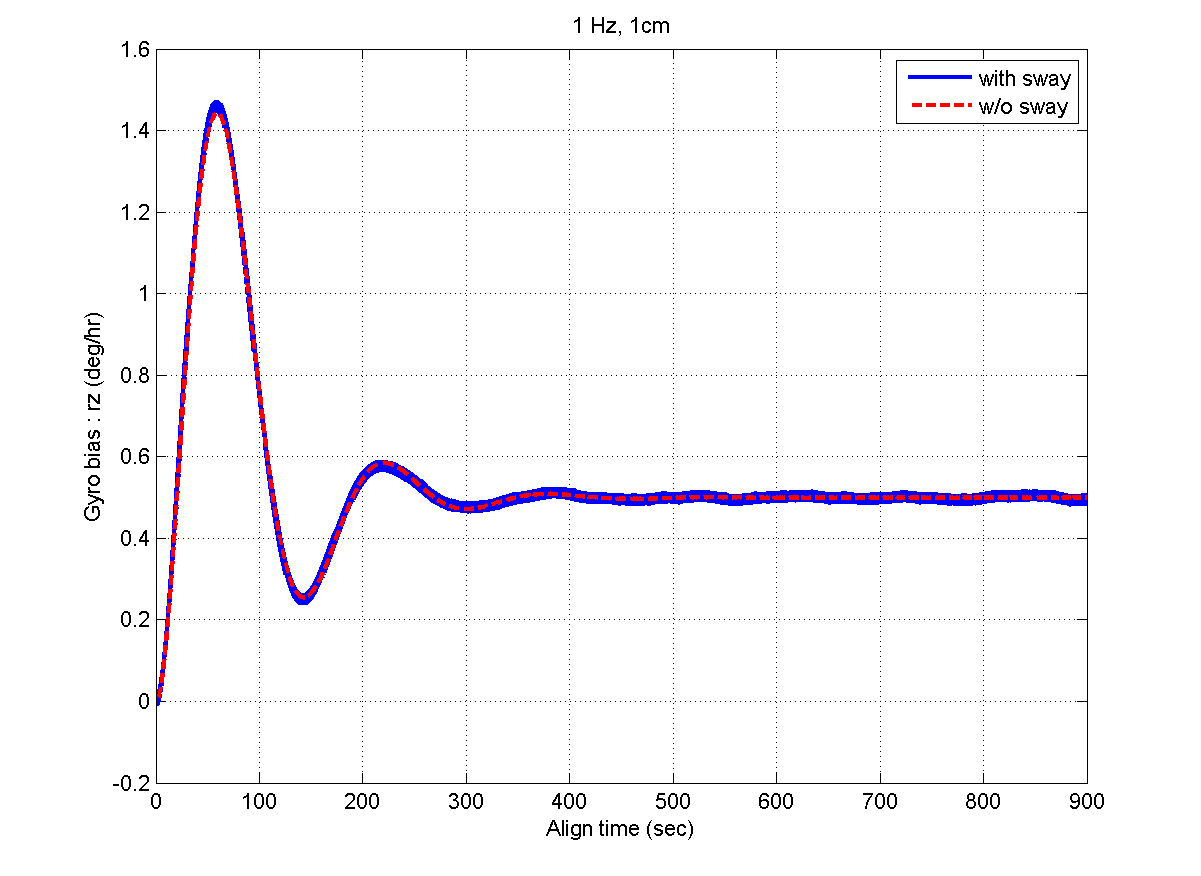
Figures 5 and 6 show the INS measurements, where the variations caused by the AF converter are noticeable. Figures 7 through 12 show the estimation results. The y- and z-axis accelerometer biases result in alignment errors of -10.31 arcsec in the pitch and 8.25 arcsec in the roll, respectively,as shown in Figs. 9 and 10. It takes about 200 seconds for the alignment errors to be settled, which results from the

selection of the filter gains in the previous section. After the steady states are reached, the estimation errors of the velocity and attitudes are within 1 mm/sec and 4 arcsec,respectively, which well satisfy the specification. Figures 11 and 12 show that the bias estimates converge to their true values. Furthermore, there are almost no differences between the results obtained in the sway condition and those in the no-sway condition. The computational time for filter processing during one sampling period of 0.01 sec is found to be 2.4 msec. The computational speed is fast enough for real-time implementation. Therefore, from the simulation results, it can be concluded that the filter well meets the required performance in terms of the alignment accuracy,convergence speed, and computational speed.

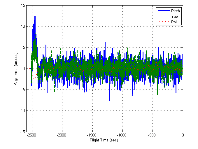
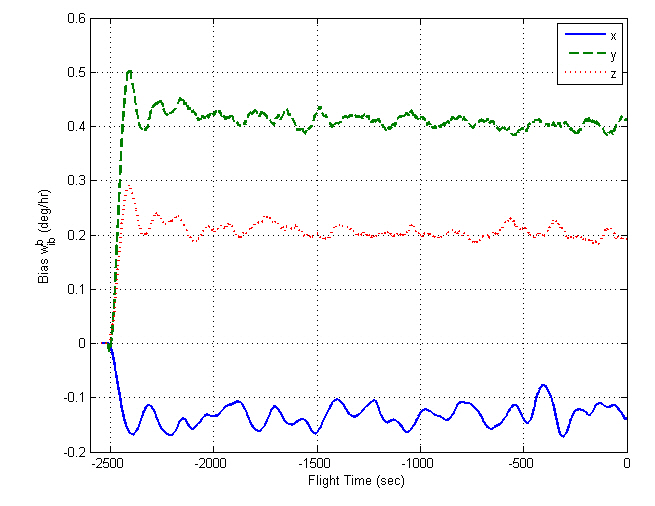
Besides the test described above, many ground-based tests have been performed before the flight test for verifying the proposed algorithm. Some kinds of test results are described in Song et al. (2009), which also includes the comparative results with Kalman filtering. Finally, the alignment filter was implemented in an on-board INS for the navigation of Naro-1, which was launched on August 25, 2009. Figures 13 through 16 represent the alignment results for the flight test.

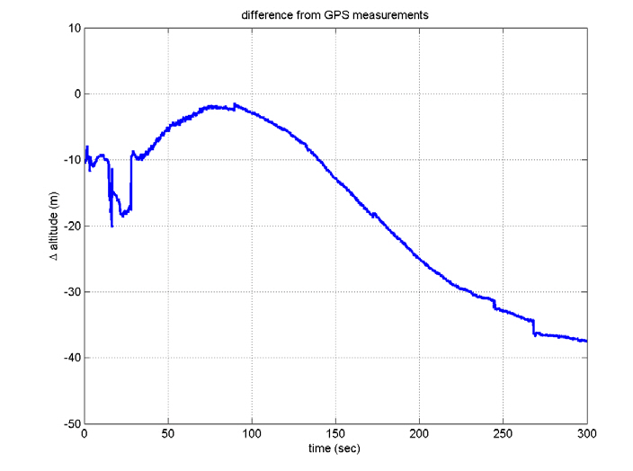
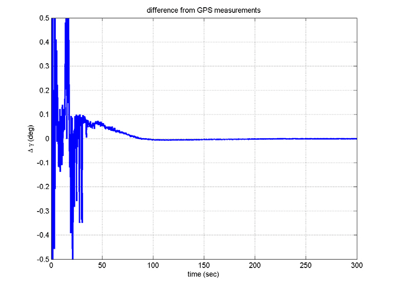
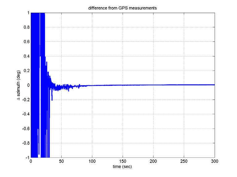
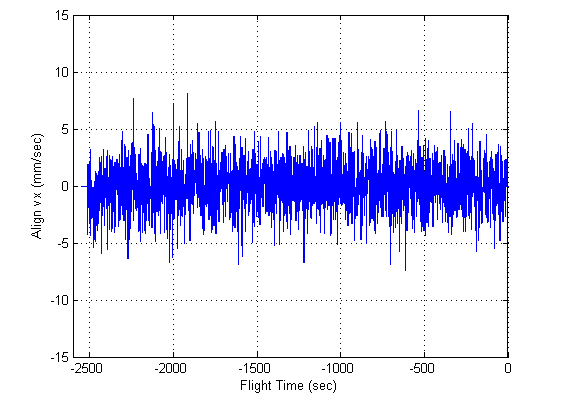
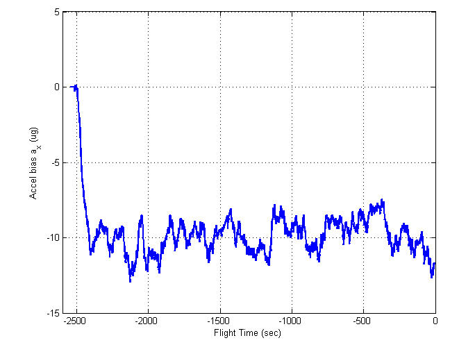
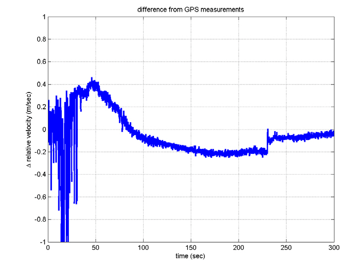
In contrast to the computer simulations, the true attitudes are not known in real flight tests. Here, the filtered residuals,viz., the values after the LPF is passed, are considered as the alignment errors, which determine the alignment performance. The alignment errors are within 4 arcsec, which satisfies the requirements, and the gyro and accelerometer biases show convergence in their specifications. Figures 17 through 20 show the INS navigation results, where they are

compared with those obtained with a global positioning system (GPS) unit. The position-determination errors of the GPS are less than 100 m (RMS), which seems to be small enough to employ the GPS in evaluating the performance of INS. Although the differences increase slightly since there are no aiding devices, they are so small. That is, the telemetry data show that the navigation using INS was successful,although the satellite did not reach the correct orbit. This indicates that INS was well aligned.

An initial fine alignment algorithm, which can be applicable to a strap-down INS for satellite launch vehicles,is developed here. Instead of Kalman filtering, a robust alignment algorithm using a simple PI-controller is designed,which can estimate all the observable error sources(alignment errors and biases). It satisfies all the requirements of the initial alignment algorithm for launchers. Its very simple filter structure allows fast computation, which also enables real-time implementation. The results of computer simulation show the robustness of the filter; its performance is still conserved in the sway condition. The performance is also proven in the Naro-I flight test, where very good navigational performance is achieved through the use of the accurate initial alignment algorithm.