Linear quadratic control (LQC) is a well-known control algorithm in the area of linear systems control. LQC originated from mean-square filtering, researched by Wiener in 1940s (Wiener, 1948). The LQC problem is based upon linear systems, and the cost function of the performance is constructed in the form of quadratic terms which track performance and control efforts. An objective in LQC entails cost minimizing, and the corresponding control input solution can be obtained by the well-known Riccati equation.In the solution procedure, various methods can be used; the Hamilton-Jacobi optimization equation is used to derive the Riccati equation.
The obtained solution provides gain-robustness and global optimality performance (Dorato et al., 1995). Additionally,because of such advantages, the LQC algorithm has been applied to various areas such as ground-vehicles, missions,aircraft, and spacecraft (Fravolini et al., 2003; Gribble, 1993;Lovren and Tomic, 1994; Plumlee and Bevly, 2004; Psiaki,2001; Ridgely et al., 1987).
The LQC solution was originally derived in a regulating problem, which is called the linear quadratic regulator(LQR). The regulating problem specifies that the desired state is zero, and the corresponding controller maintains the vehicle state at zero. To apply the LQC solution in a tracking problem, which has a non-zero desired trajectory, the disturbance-rejection problem was considered by modifying system dynamics (Anderson and Moore, 1990; Dorato et al.,1995).
This study proposes a control algorithm that adds collision avoidance to the original LQC tracking problem. To achieve this goal, an additional term is inserted into the cost function to account for a collision avoidance effect. A detailed derivation of the proposed algorithm is introduced in Section 3. One of the important changes in the new approach is the off-diagonal term of the weight matrix on state. This term is not zero, which is a measure taken in order to implement the collision avoidance constraint. To prevent equalization of the position between vehicles, the cost function should consider the correlation and dependency between state variables. As a result, the weight matrix on states becomes a non-diagonal matrix, which is easy to implement by using commercial software tools such as MATLAB.
After performing the derivation of the optimal control history for a multiple-vehicle case, the proposed algorithm is applied to a satellite formation flying (SFF) mission. SFF is a combined phrase consisting of the words satellite and formation flying. SFF has recently received much attention(Clohessy and Wiltshire, 1960; Hadaegh et al., 2000;McCambish et al., 2009; Speyer, 1979; Xing et al., 2000).As with other concerning satellite missions, all guidance,navigation, and control theories are necessary for SFF.Additionally, among guidance and control parts, the collision avoidance problem is an important issue because multiple satellites are operating.
Many researchers have studied the collision avoidance problem in SFF. Slater et al. (2006) referred to the collision probability function, and used an impulsive control to maintain a safe distance between spacecrafts. Wang and Schaub (2008) attempted to avoid collision using electrostatic (coulomb) forces with a Lyapunov-based control law. And, Lim et al. (2005) used potential functions to prevent collision. This paper proposes a collision avoidance algorithm by modifying the original LQC tracking problem.The conventional LQC provides desirable qualities such as gain-robustness and optimality; these properties can be preserved in the proposed algorithm because the proposed algorithm is based on the LQC problem. In addition, an optimal solution can be obtained by simple numerical integration only.
This paper is presented in the following manner. In Section 2, introductory material of LQR is presented. The main control algorithm and its derivation are introduced in Section 3. Finally, the algorithm’s application to SFF with numerical simulation is discussed in Section 4.
2. Linear Quadratic Control Algorithm
In this chapter, the LQC problem is briefly reviewed.Before proceeding, the general LQR algorithm including disturbance rejection will be introduced. In the next chapter,a collision avoidance measurement term is augmented to the linear control framework introduced here.
2.1 Linear quadratic regulator
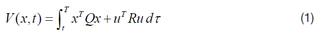
The LQC problem originated from a mean-square filtering algorithm by Wiener. The LQC algorithm manages a linear system, and its performance is measured in quadratic form.A linear system is a system in which the system equation is constructed by linear operators. Quadratic form indicates cost terms, like the tracking performance of states and control effort of an actuator, are represented by the quadratic errors.
where
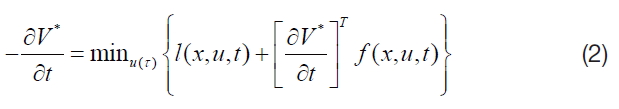
The above equation is the Hamilton-Jacobi optimization equation. Additionally,
Firstly, we will consider a simple case, where


2.2 Disturbance rejection problem
Disturbance rejection problems are characterized by an additional disturbance term

In addition, the disturbance rejection problem is similar to the tracking problem. The tracking problem requires a nonzero desired state,
3. Collision Avoidance Consideration
In multiple vehicles control, such as airplanes and spacecrafts, collision between each vehicle should be avoided. This avoidance guidance is known as ‘Collision Avoidance’, and associated research has been conducted for many years. In this chapter, an additional cost term will be added to the pre-defined cost function
The regulating problem, which is when
To add the collision avoidance effect into multiple vehicle guidance, we will augment additional cost terms to the cost function,
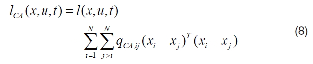
where
For a simple case, the number of vehicles is assumed to be two, which means
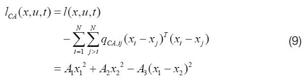
where
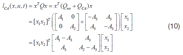
where
This sub-chapter investigates the tracking problem. As noted before, the tracking problem has a non-zero desired state
Firstly, for simplicity, it is assumed again that there are two vehicles, and they move along a one-dimensional axis. Four state variables represent the system status as before. However, the vehicles’ tracking errors from the desired trajectory ξ
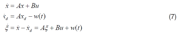
However, the vehicles’ tracking errors from the desired trajectory ξ(t)=x(t)-xd(t) is adopted as state variables, rather than the vehicles’ positions and velocities directly. The tracking problem can then be converted into a regulating problem as given by Eq. (7). And, a new state representing the tracking error becomes ξ(t)=[x1-x1d x2-x2d x˙1-x˙1d x˙2-x˙2d]T .
Because state variables are different, the cost function
where x1d
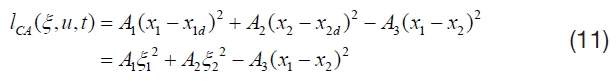
In Eq. (11), it should be noted that the last term, which is used to prevent collision avoidance, has a quadratic form with a negative sign. This form is must be applied to the original LQC algorithm which is derived in a quadratic manner. In general collision avoidance research, rather than a quadratic term, an inverse of the distance term like (xi?xj)?1 or a potential function with an exponential term is used to prevent collision. In this manner, collision could be avoided regardless of the shape of the desired trajectory. However, an optimal property such as the minimizing control effort is hard to obtain when those terms are used. In addition, if optimal equations could be constructed, the equations are not easily solved. In this paper, the proposed algorithm does not guarantee collision avoidance for some cases in which different trajectories or systems are desired, and confirmation of the obtained control input could be needed. However, the proposed algorithm is based on the conventional LQC problem, so the proposed algorithm inherently preserves gain-robustness and optimality, and an optimal solution can be obtained by simple numerical integration.
We can see that Eq. (11) is similar to Eq. (9) which was derived in the regulating problem. But, different in state variables exist. The x1, x2 terms in Eq. (9) are replaced by ξ1=x1?x1d, ξ2=x2?x2d in Eq. (11). Because of this change, the cost function with tracking problem, Eq. (11), cannot be formed with quadratic terms, ξT
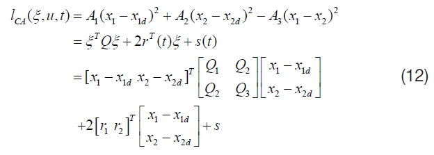
where
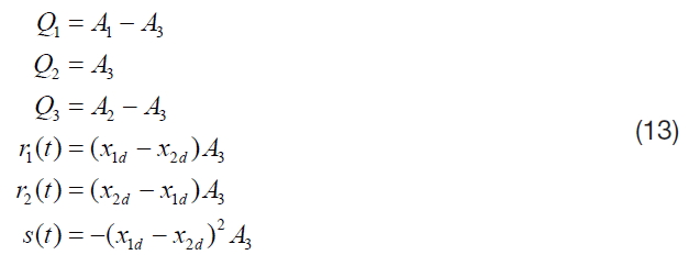
From Eq. (12) and Eq. (13), one can express the collision avoidance effect as a combination of a matrix and vector. Finally, the optimal input history is derived using the Hamilton-Jacobi optimization equation, Eq. (2). Because this problem manages the tracking problem, the following form for the performance measure is introduced, i.e.,
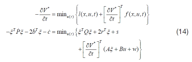
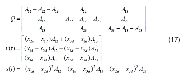
After expanding the above equations and collecting the quadratic terms, linear terms and state-independent terms respectively, the results can be summarized as,
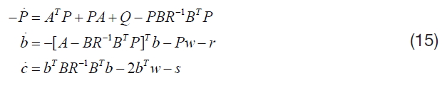
where
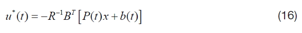
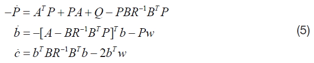
Eq. (15) shows similar results to the original disturbance rejection solution, Eq. (5). A comparison of the two results is summarized in Table 1. One can see that there is an additional term ?
Until now, cases involving two-vehicles have only been considered, rather than the multiple-vehicle cases in which N≥3. However, we can generalize the results of the above sub-chapters into a multiple vehicle case without complex derivation.
Firstly, note that the solution for the performance measure coefficients
To visualize the tendency of the change in
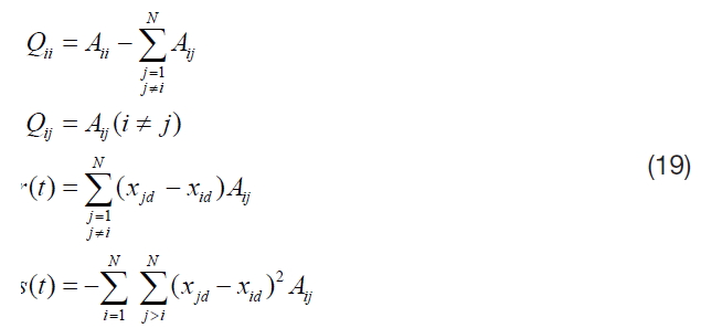
Finally, a generalized form of the multiple-vehicle case can be obtained, as shown in Eqs. (18) and (19).
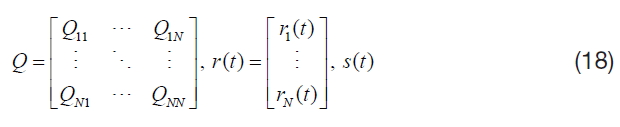
where,
3.4 Example: simple 2-dimensional tracking problem
Before applying the derived control algorithm to real practical problems, such as SFF, a simple problem is analyzed to demonstrate the validity of the control law. In a two-dimensional space, two-vehicles are used, requiring no additional forces except control acceleration
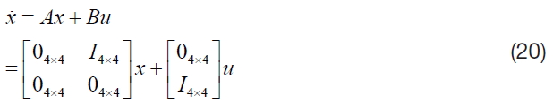
where x=[x1 x2 y1 y2 x˙2 x˙2 y˙1 y˙2]T and
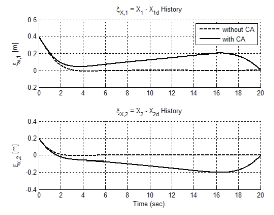
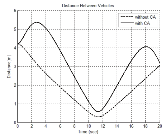
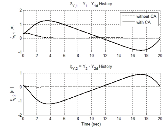
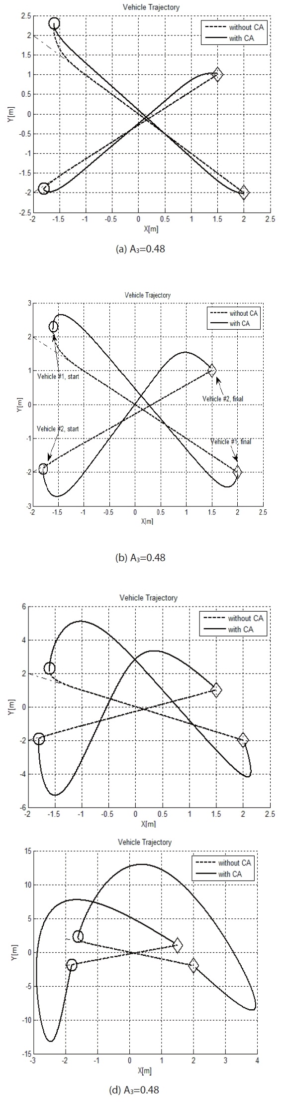
Figures 1-4 display the simulation results of this condition. Fig. 1 shows a vehicle trajectory from its initial position to the final position. The solid line represents a trajectory with the original tracking algorithm, and the dashed line represents the trajectory with the derived algorithm, considering collision avoidance between the vehicles. To prevent collision between vehicles, vehicles do not follow a pre-determined desired trajectory. In Fig. 2, one can confirm that the distance between vehicles becomes larger when collision avoidance is added. In addition, Figs. 3 and 4 show corresponding tracking errors between the present position and the desired trajectory.
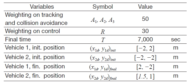
[Table 2.] Simulation parameters

Simulation parameters
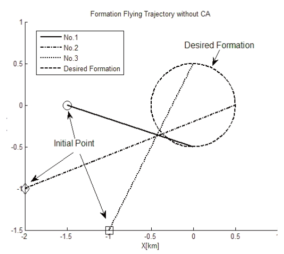
Figure 5 shows the change of vehicle trajectory as the collision avoidance weighting parameter
vehicles tends to become longer in the time history.
In this chapter, the control law derived in the previous chapter is applied to a SSF problem. SSF has been investigated for many years, and the Clohessy and Wiltshire (CW) equation is generally employed as the linearized equation for relative dynamics. By using the CW equation, an application of collision avoidance algorithm is demonstrated, and the corresponding simulation results are presented.
4.1 Relative equations of motion
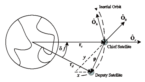
SSF is commonly constructed by a chief satellite and a deputy satellite. The amount of deputy satellites present can be more than one, and the actual number is determined by mission characteristics. The coordinated frame (localvertical-local-horizontal [LVLH] frame) has an origin at the center of the chief satellite and the direction of each axis is drawn in Fig. 6. The

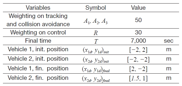
[Table 3.] Simulation parameters

Simulation parameters
where
Eq. (21) has non-linear terms such as a square term. CW developed a linearized equation of Eq. (21) using assumptions such that the chief satellite travels in a circular orbit (Clohessy and Wiltshire, 1960).
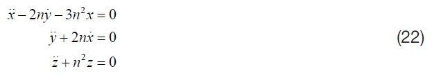
Eq. (22) is the CW equation, also known as Hill’s equation. In Eq. (22), the term stands for the angular rate of the chief satellite. Using the linear equation of SSF, CW equation, one can apply the derived linear control algorithm that were presented in the previous chapter.
The application of the linear optimal control algorithm derived in the previous chapter is explored in this sub-chapter. A two-dimensional space,
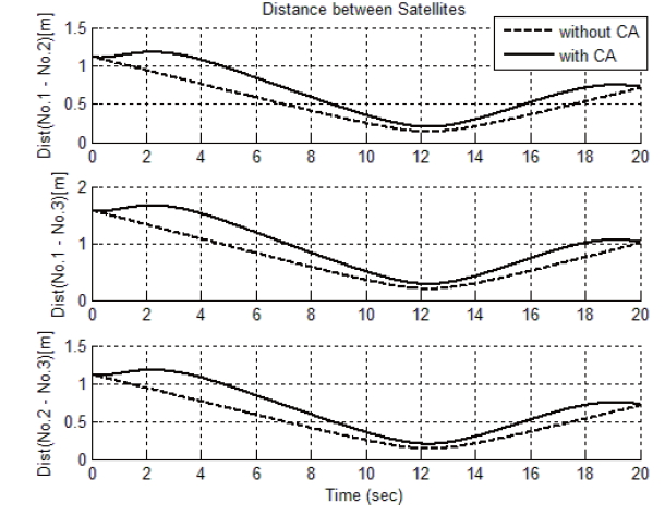
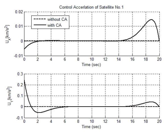
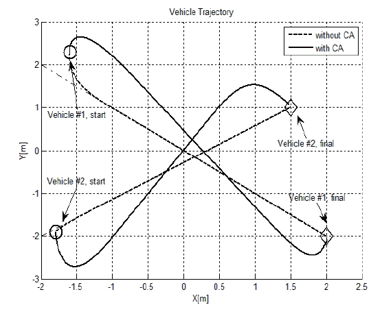
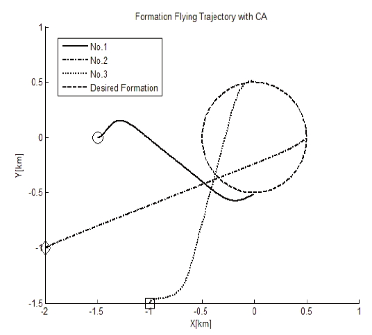
Details for the cost function coefficients and the initial condition of each satellite are presented in Table 3. Figures 7-10 represent resultant plotting of the SSF control simulation. Figure 7 presents satellite trajectories from initial positions to final mission destinations. No weighting term was added for the collision avoidance in the Fig. 7 simulation, but Fig. 8 considers collision avoidance for trajectory generation. In Fig. 8, satellites enter the final circular formation by detouring non-direct guidance as Fig. 7, to prevent collision between satellites.
Figures 9 and 10 present the corresponding distance between satellites as well as the acceleration input. Figure 9 shows the distance between each satellite, which is
In this paper, a linear control algorithm was derived for the tracking problem by solving the Hamilton-Jacobi optimization equation. To avoid collision between vehicles, an additional weighting term was introduced when constructing the cost function. The corresponding optimal control solution maintained a similar form as the original LQR tracking problem, which does not consider collision avoidance. The only difference was that extra terms were added in the differential equations of the performance measure coefficients. After deriving the control history solution, a simple example involving two vehicles was considered. In addition, the application of the control algorithm to SSF mission was analyzed, and numerical simulation was presented. Using this proposed algorithm, SSF problems as well as other problems involving multiple-vehicles could consider collision avoidance in the tracking problems.