Economic growth is associated with high energy consumption.In Korea, due to industrialization, the demand for energy increased rapidly in the 1970s. In particular, electricity consumption increased by about 9.6% per year from 1980 to 2005. Korea’s high energy consumption was strongly related with the rapid expansion of industrial sectors [1, 2].

Higher energy consumption by industries requires greater energy generation. In general, greenhouse gas emissions (GHGs) are linked with the consumption of energy. Although there is a relationship between energy and GHGs, there is nothing that signifies the proportion in term of quantities, as different fuels have different global warming potential factors. To meet the challenge of climate change due to the greenhouse gas effect,identification of emission sources is regarded as a highly desirable task, which would give direction on how to reduce this effect. To manage this assessment, as well as understand the energy consumption behavior of each sector, an appropriated tool is required. In the present study, an input-output analysis of the national economy was conducted to provide the predominant characteristics for identifying all the upstream economic inputs to the industrial sector to which they apply. The input-output analysis, developed by W.W. Leontief, studies the relationships between economic sectors [3, 4]. The fundamental information used in the input-output analysis was related to the flow of products from each industrial sector, which were considered the producer, to each of the sectors, both internally and externally, which were considered the consumers. The aim of applying an input-output analysis is to quantify the total amount of energy required for one financial unit of production by a given sector.

The main equation of the input-output model is shown in Equation (1):

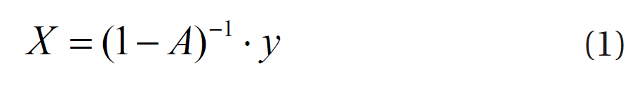
where x is the vector of the required input, I the identity matrix containing one (1) in each diagonal element and zero in all other elements, and A the input-output direct requirement matrix,which represents the direct requirement coefficient, aij, denoting the input of a product from the ith row used by the jth column to make a unit output for the jth column. The factor (I-A)-1 is generally known as Leontief inverse coefficient, which refers to the amount of product both directly and indirectly required to fulfill a unit of final demand for that product.

Miller and Blair [4] developed an input-output model for application to the energy sector during the oil crises in the early 1970s, which has been used to analyze the relationships between energy and climate change. Mayer [5] calculated and analyzed a hybrid energy input-output table of the Germany economy for the years 1995, 2000, 2002, 2003, and 2004. Park and Heo [6] quantified the direct and indirect energy requirements of a household in the Republic of Korea. Their study applied an input-output analysis and used a relatively disaggregated inputoutput table for the nation over the period 1980 to 2000. Nguyen[7] examined the impacts of increasing the electricity tariff

on the long run marginal prices of other products in Vietnam using a static input-output approach. Yoo and Yoo [8] applied an input-output framework to investigate the role of nuclear power generation in the Korean national economy. Acquaye and Duffy [9] estimated the energy and GHG emission intensities relating to Irish construction and its subsectors, and found the contribution to the Irish national emissions using an inputoutput analysis. Mu et al. [10] developed an input-output table of electricity demand based on the Chinese national economy.Their methodology was designed to identify key sectors for final energy consumption. Baral and Bakshi [11] proposed and demonstrated the use of a thermodynamically augmented economic input-output model of the US economy for obtaining sector-specific energy to money ratios.

According to previous investigations in the available literature, a few studies have used energy input-output tables to quantify the energy structure and identify the causality between the energy supply and demand sides. To be more proactive about energy management, in accordance with the rapid growth in demand, the correlation between supply and demand, in term of energy units, including the decomposition of its structure,should be investigated. This paper; therefore, attempted to address the relationships between the energy demand and supply for fifteen industrial and non-industrial sectors. For this, an energy input-output table was initially constructed,with a mathematical approach simply demonstrated. A sensitivity analysis was then conducted by quantifying the significant contributions from each sector. An uncertainty analysis on the CO₂ emissions was also evaluated to communicate the reliability of the result. The Monte Carlo simulation was used as the procedure for this evaluation.

The objective of this work was to quantify the structure of energy demand and supply for industrial and non-industrial sectors in South Korea for 2005, and demonstrate the CO₂ emissions caused by the demand side compared to the supply side.

Two main primary sources were data from the energy balance of 2005, surveyed by the Korea Energy Economics Institute(KEEI) [12, 13], and the conventional input-output table of 2005,prepared by the Bank of Korea [14] in 2008.

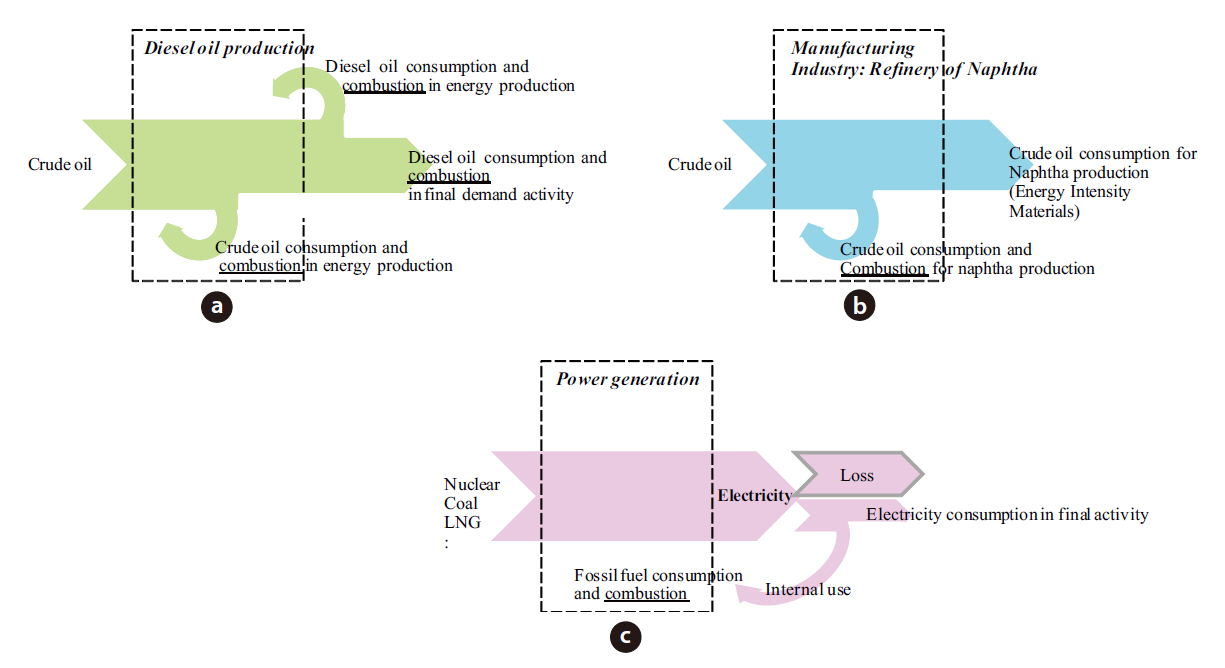
In the initial energy input-output construction, definitions of the energy and GHGs terms, and their conditions of use were required for this work to consistently determine the total energy consumption and GHG emissions for the economy. Energy was measured as the consumption of primary, secondary and tertiary energies, while GHG emissions were measured as the combustion of primary and secondary energies. Generally,the consumption of energy by industry is for processing; otherwise it is used for material transformation; for instance, the production of naphtha from crude oil. Therefore, it is important to distinguish between the processing and material transformation use of energy in an industrial activity, because the main factor influencing the quantification of CO₂ emissions from an industrial activity is the combustion of energy. Fig. 1 illustrates three different features of energy consumption in processing and transformation, and the resultant CO₂ emissions.

Fig. 1(a) shows the consumption and combustion of crude oil in the production of diesel oil. Diesel oil, as a product, is further consumed and combusted as a final demand within both industrial and non-industrial sectors. Fig. 1(b) shows the consumption and combustion of crude oil in the process of naphtha production. It also indicates that crude oil is consumed and transformed to naphtha, without any CO₂ being emitted.Fig. 1(c) involves the generation of electricity. Primary and secondary energies are consumed and combusted during power generation. Thus, CO₂ is emitted only during the energy production stage. Electricity is then distributed as a final demand.Furthermore, electricity is used internally in the production process of power generation. With respect to energy processing,the scope of the collected data was for the South Korean operation;hence, the resultant environmental load was excluded as an import.

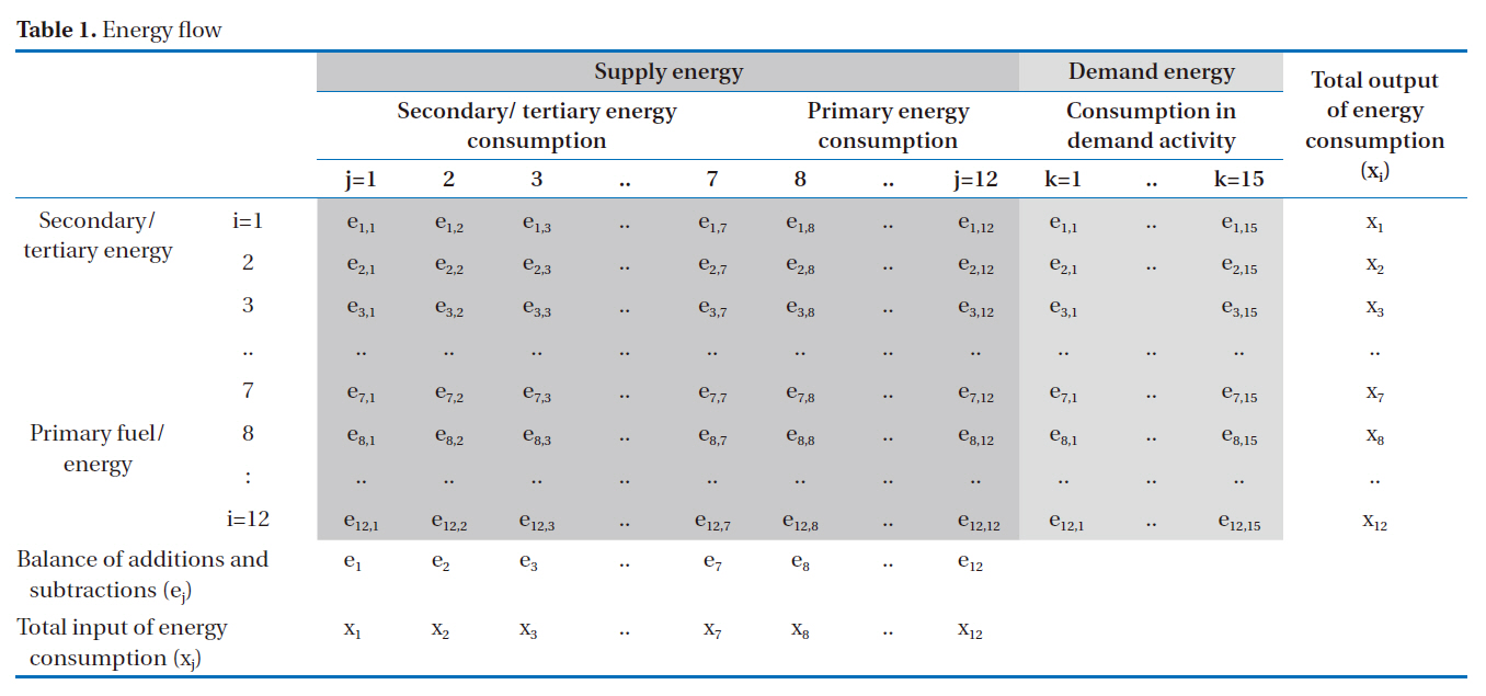
The energy input-output table used in this study was constructed by integrating the conventional input-output data of 2005, developed by the Bank of Korea in 2008, and the energy consumption by industry, as investigated by the KEEI. Tone of oil equivalent (TOE) is the physical unit expressed in Table 1. To be able to better track the energy flow from a demand and supply perspective, it is worthwhile considering the energy sectors separately from the industrial and non-industrial sectors when forming the input-output table. The energy supply table presents the transaction of energy between 12 rows and 12 columns for the energy sectors, which are coal, crude petroleum, natural gas, nuclear, renewable energy, coal product, fuel oil,other petroleum product, non-fuel oil, gas, heat and electricity. The numbers between the rows and columns indicate the amount of energy from the i^th row consumed to produce a unit of energy output for the j^th column. The industrial table addresses the amount of energy demand from the i^th row consumed by the k^th column to make a unit output of industrial or non-industrial activity. For the fifteen industrial and non-industrial sectors categorized in this study, the information on energy demand provided by the KEEI were agriculture and fishery, mining, food and tobacco, petrochemical (processing base), petrochemical (material base), iron and steel (processing base), iron and steel(material base), non-metallic metal, non-ferro, textile and wood product, fabricated metal, manufacturing, construction, trans-

portation, residential, commercial and public, and others.

To prevent errors when accounting for the CO₂ emissions, the transaction number for communicating between rows and columns should indicate whether fuel or energy is used for processing or transformation. Referring to the 2006 Intergovernmental Panel on Climate Change (IPCC) Guideline; in many cases, the exact fuels used in refineries to produce the energy required to operate the refinery process are not easily derived from the energy statistics, but have been typically estimated as 6 to 10 percent of the total fuel input to the refinery. In this case study, 10 percent was employed as the fuel input for running the petroleum energy process. This approach and the percentage of fuel input for running the process were applied for coal products also. The petrochemical product was disaggregated into the processing and material bases in order to prevent an error in the CO₂ analysis. Similarly, the iron and steel sector was also divided into processing and material bases for the purpose of energy consumption. The energy input-output table is presented schematically in Table 1.

e^st _i,j illustrates the amount of secondary or tertiary energy from row ‘i’ consumed to produce energy column ‘j’, e^st _i,j refers to the amount of energy from row ‘i’ consumed by industrial activities ‘k’, e^p _i,j is the primary energy ‘i’ burned to produce energy ‘j’, x^st ₁ represents the total consumption of secondary or tertiary energy type ‘i’ or consumed by industrial sector ‘k’, and x^p _i shows the total consumption of primary energy type ‘i’.

A mathematical model was initiated from the concept of energy balance. From Table 1, the total energy consumption associated with national activities is given by the sum of different energy productions and industrial consumptions.

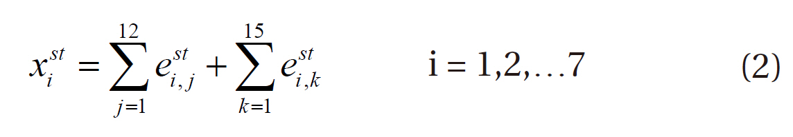
The normalization energy term representing the input energy

from row ‘i’ deliver to produce a unit of output energy in column‘j’ was defined as:

Substituting Equation (3) into Equation (2) results in the following:

Reorganizing gives the following equation:

which can be written as a matrix:

where X^st is the vector of x^st_i, I the unit matrix, G^st the matrix of the summation of g^st _i,j , (I ?G^st )^-1 the inverse matrix of (1-g_i,j )^-1 , and E_k the matrix summation of e_i,k.

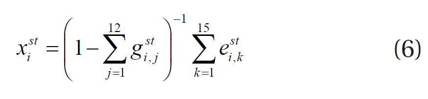
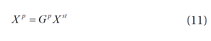
With Equation (7) the required quantities in total of secondary or tertiary energy, x^st , to satisfy the final demand of ‘E’ units by industrial sector ‘k’ can be calculated. This equation can also be used to analyze the relationship between energy supply and demand from industrial and non-industrial sectors, i.e., the impact for such a change in energy technology production,measured in mass units (for example renewable energy used in electricity generation), on the total energy consumption and CO₂ emissions of the demand sector and vice versa, can be assessed. Analogously, the total amount of primary energy, x ^p , can be calculated, as shown in Equation (8).

Typically, primary energy is used to produce secondary or tertiary energy, instead of being directly consumed during an industrial activity; hence, the second term on the right hand side can be neglected. The coefficient , g^p _i,j , which reflects the amount of primary energy input ‘i’ required to produce x^st type ‘j’ per total output of x^st, is given in Equation (9), with the result obtained shown in Equation (10).

Substituting Equation (9) into Equation (8), gives:

which can be written as a matrix:

where X^p is the matrix of x^p_i, G^p the matrix of the summation of, g^p _i,j , and X^st the vector of x^st_i.

Replacing x^st _i from Equation (7) yields:

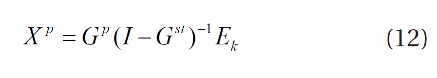
This equation gives the total primary energy required to produce the secondary or tertiary energy required as a final demand.

In summary, Equations (7) and (12) provide the mathematical formula for determining the total annual energy consumption of each energy type for the industrial and non-industrial sectors.

2.6. Productiveness Condition

A productiveness condition check is needed when an input-output analysis is performed. The Leontief inverse matrix (1-g^st_i )^-1 performed in this study meets the requirements of the Hawkins and Simon (H-S) condition, once all the minor principals of the determinant (1-g^st_i) have been proved positive:

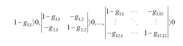
(Modified from Nakamura and Kondo, 2009 [15])

This current section presents the results of the model calculations for the net energy consumption and CO₂ emissions of the fifteen industrial and non-industrial sectors. With respect to the energy consumption, the results of energy demand and supply,including the structure, are shown in Fig. 2. Using the CO₂ factors from the IPCC, the CO₂ emissions on a yearly basis for each sector are illustrated in Fig. 3.

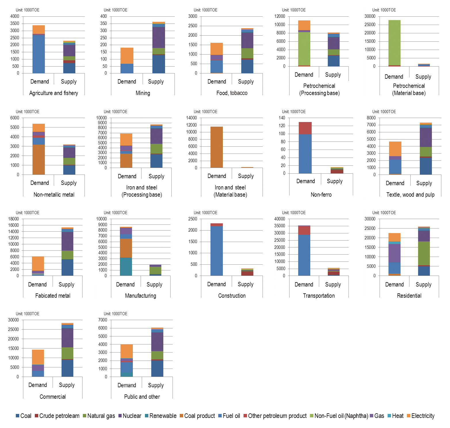
The results in Fig. 2 show the demand and supply energies consumed by fifteen industrial and non-industrial sectors. In addition to the current study, one advantage of developing an energy input-output model is that it offers a better evaluation of the energy structural decomposition analysis affected by the choice of energy from either side of the energy demand or supply. Fig. 2 shows the structure of the demand and supply energies,which were divided into 12 types of energy for all sectors.

To deliver an energy demand of 3.3 million TOE required by the agriculture and fishery sector, a supply energy of 2.31 million TOE is required for its production. For the mining sector, a total supply energy of 0.36 million TOE is needed to satisfy the demand energy for electricity (orange color) of 0.11 million TOE and fuel oil (blue color) of 0.067 million TOE. For the food and

tobacco sector, the demand and supply energies are 1.62 and 2.40 million TOE, respectively. For the petrochemical product sector (purpose in processing), the results indicated that 11.07 and 8.19 million TOE of energy were consumed for demand and supply activities. In the case of the petrochemical product sector (purpose in energy transformation to material), non-fuel oil (green color) of 27.2 million TOE and other petroleum products (red color) of 0.78 million TOE accounted for the vast majority of directly required energy transformation. To acquire this amount of non-fuel oil and other petroleum products (LPG), 1.5 million TOE in total are used in energy production. In the case of the non-metallic metal sector, coal as a product (brown color) plays a key role for the demand energy, accounting for 3.17 million TOE. Fuel oil of 0.77, electricity of 0.85, gas of 0.36 and other petroleum product of 0.24 million TOE are also required for this sector. In addition, a total of 3.22 million TOE would be needed to supply energy used by this sector. For the iron and steel sector (purpose in processing), a total energy of 6.89 million TOE are consumed by demand activities, for which coal product and electricity are mainly used. The energy supply is considerably higher than the energy demand, which is 8.76 million TOE.

Meanwhile, the energy demand for the iron and steel sector (purpose in energy transformation to material) is completely met by coal product, accounting for 11.57 million TOE. To produce this amount of coal product, about 0.18 million TOE is needed as supply energy. Comparison of the energy demand and supply for the textile and wood product sector, the amount of demand energy, which is 4.691 million TOE, is relative small compare to supply energy accounting for 7.34 million TOE. The total energy demand delivered to the fabricated metal sector is 6.15 million TOE, while supply energy which is higher than demand energy is 15.31 million TOE. The structure of energy demand and supply

for the construction sector was similar to that for the transportation sector, but with a slightly different amount of consumption. A similar picture, high energy supply, but low demand, was projected for non-industrial, residential and commercial, including the public and other sectors. The results obtained revealed that the choice of energy on the demand side influences the type and amount of energy on the supply side and the total consumption.

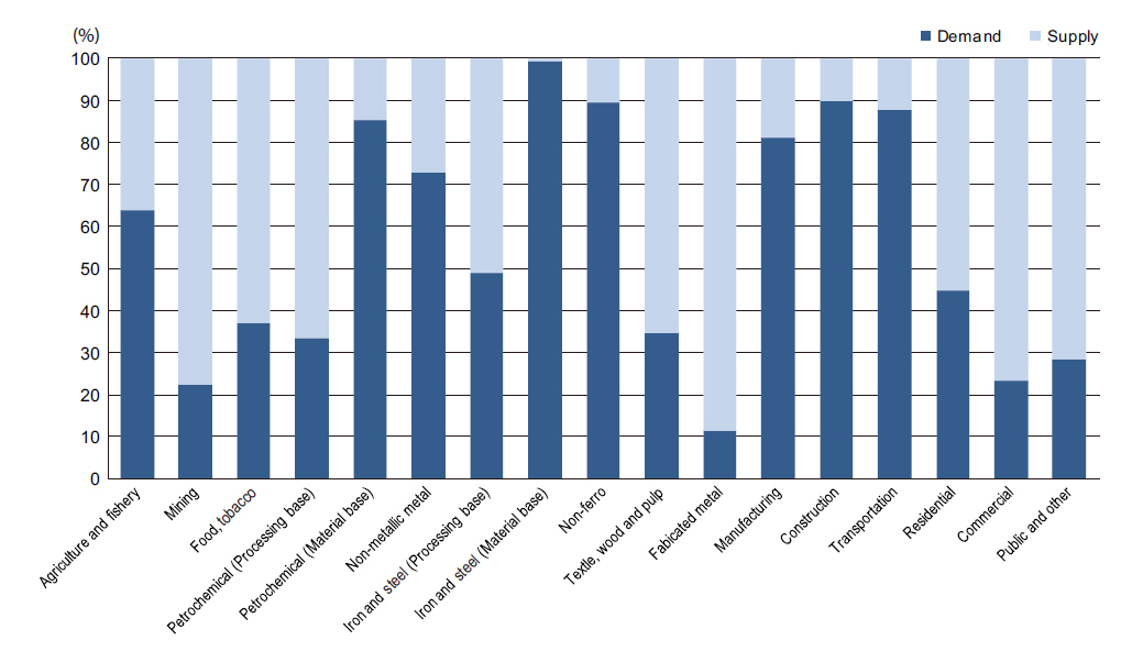
The most important indicator typically used connected with energy consumption is the CO₂ emissions. The emission factors of CO₂, CH₄, and N₂O for CO₂ equivalents (eq.) for each fuel type mainly refer to the 2006 IPCC [16] guideline for stationary and mobility combustion. The results from the model calculation were multiplied by the CO₂ intensities vector. The corresponding tons of CO₂ eq. emitted by each sectors were presented accordingly. As mentioned earlier, the contribution of energy to CO₂ emissions is only from combustion. In the graph, given in Fig.3, the CO₂ emissions from the demand side are shown relative to the CO₂ from the supply side for each sector.

From Fig. 3, the CO₂ emissions incurred by the supply of energy to the industrial sectors of mining, food and tobacco,petrochemical processing base, iron and steel processing base, textile and wood, fabricated metal, residential, and commercial,including public and others, were observed to be particularly high compare to those due to energy demand. CO₂ emissions (from the industrial and non-industrial point of use), which accounted for more than 70% of the total emission, were found for the petrochemical material base, non-metallic metal, iron and steel material base, non-ferrous, manufacturing, construction and transportation sectors. Indirect CO₂ emissions (from the energy combustion at energy production) play a dominant role,accounting for 70% of the total for the mining and fabricated metal sectors and for non-industrial purposes of the commercial and public sectors. The indirect CO₂ emissions for the agriculture and fishery sector were 38%, with 50% for the iron and steel (processing base), 65% for the textile, wood and pulp sector, and about 55% for non-industrial purposes within the resident sector.

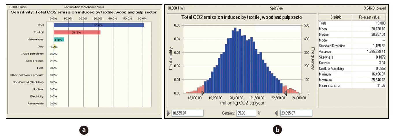
This section attempts to address the most influential parameter on the emission results and determine the reliability of the results with respect to the uncertainty of the input parameters.Therefore, a Monte Carlo simulation, using the Crystal Ball software, was employed. Initially, the input parameters had to be specified for the uncertainty distribution. The Batch Fit tool contained within Crystal Ball was employed to obtain the best fit probability distribution for each piece of technical datum (Crystal Ball, 2008). A lognormal distribution has been found to be the most appropriate, and was selected for the current work. The total number of trial runs conducted via the Cristal Ball software was 10,000. The following figures show an example of the Monte Carlo simulation results associated with the sensitivity and uncertainty, and include the distribution for the textile, wood and pulp sector. In Fig. 4(a), the most important parameter, about 60.6%, was coal, with over 30% for fuel oil. The remainder was attributed to 6.8% natural gas, 1% gas, 0.2% crude oil, and 0.1% coal product. In Fig. 4(b), the mean total emissions of this sector per year were 20,720 million kg CO₂-eq., with a standard deviation of 1,155.52 million kg CO₂-eq. The uncertainty value described by the standard deviation divided by the mean is a term that indicates the reliability of the result. From the evaluation,the uncertainty, or the coefficient of variation (CV), was 0.0558 (5.58%). Fig. 4(b) also depicts the distribution of CO₂ emissions caused by this sector. The x-dimension provides the CO₂ emissions per basis and the y-dimension shows the probability for each value towards the total CO₂ emissions. The certainty values at the 95% certainty level ranged from 18,555.07 to 23,095.67 million kg CO₂-eq.

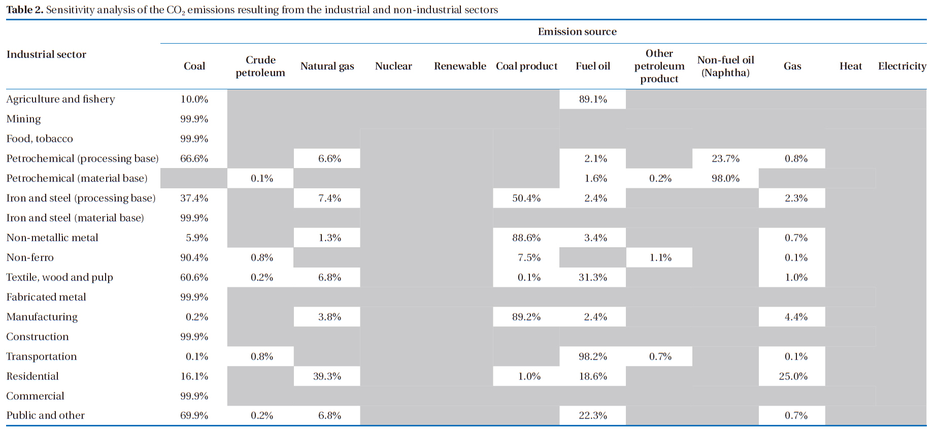
The same procedure was implemented for all sectors in the current study, as presented in Table 2. Using a sensitivity analysis,the energy type influencing the CO₂ emissions from each industrial sector can be obtained.

In the case of the agriculture and fishery sector, the main sources of emissions were fuel oil and coal, which contributed 89.1 and 10%, respectively. The major emissions from the mining sector were due to coal energy, with a percentage of about 99.9%. The contributions from the other energy sources were negligible. The same results were obtained for the food and to-

bacco, iron and steel material base, fabricated metal, construction,and commercial sectors. In the petrochemical product processing base, coal energy generated the largest quantity of emissions, contributing 66.6%. The emissions from non-fuel oil energy, natural gas, fuel oil and gas were 23.7, 6.6, 2.1, and 0.8%, respectively. The total emissions from the petrochemical product material base were mainly from non-fuel oil, accounting for 98%, fuel oil 1.6%, other petroleum products 0.2% and crude petroleum 0.1%. The significant contributors for the iron and steel processing base sector were coal product and coal energy, accounting for 50.4 and 37.4%, respectively. The major contributor to the emissions for the non-metallic metal sector was coal product energy (88.6%). Coal energy was also the main contributor for the non-ferro sector, at 90.4%. The most relevant source of emission for the manufacturing sector was coal product energy, accounting for 89.2%. Over 98% of the contribution for the transportation sector was from fuel oil energy. The total emissions of the residential sector were mainly induced by natural gas, gas, fuel oil and coal energy, at 39.3, 25, 18.6 and 16.1%, respectively. The relative importance of the emissions related to the public and other sectors were from coal energy and fuel oil, at 69.9 and 22.3%, respectively.

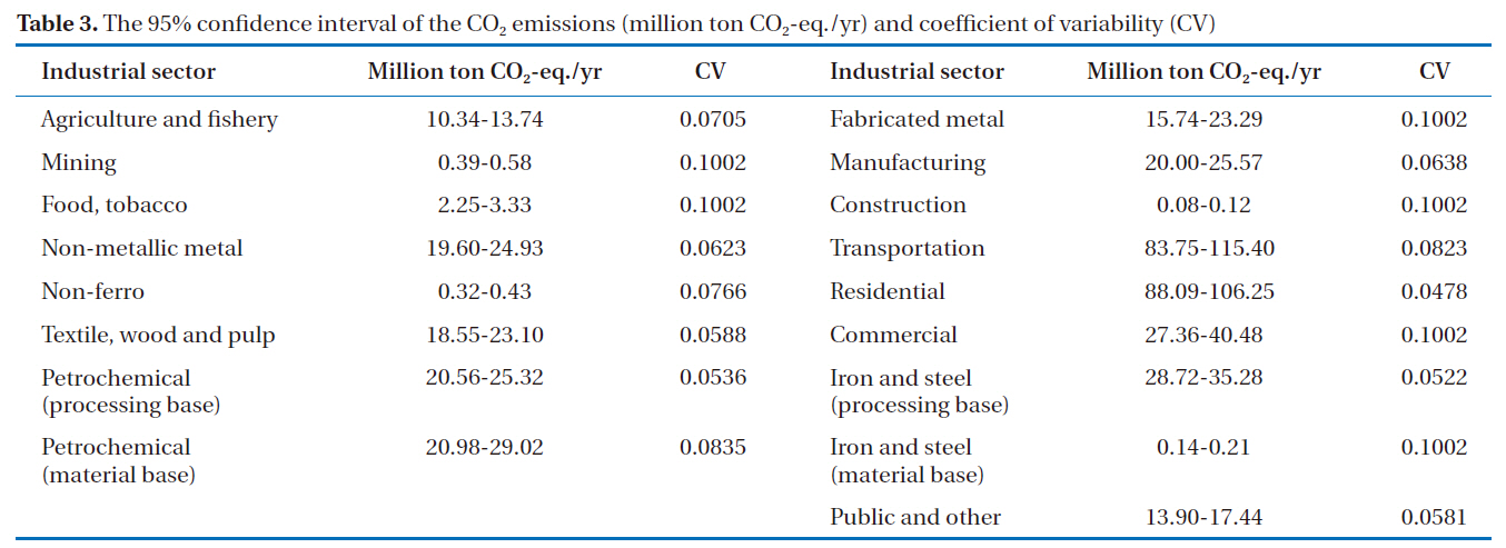
The CV, used to indicate the reliability of the results, and 95% confidence interval for all the industrial and non-industrial purpose sectors are presented in Table 3.

On an annual basis, the 95% confidence interval of the CO₂ emissions were obtained, which are shown in Table 3 for the industrial and non-industrial sectors. The results were 10.34 to 13.74 million ton CO₂-eq. for the agriculture and fishery sector, 0.39 to 0.58 million ton CO₂-eq. for the mining sector, 2.25 to 3.33 million ton CO₂-eq. for the food and tobacco sector, 19.60 to 24.93 million ton CO₂-eq. for the non-metallic metal sector, 18.55 to 23.10 million ton CO₂-eq. for the textile and wood product sector. The results for the petrochemical product processing and material bases were 20.56 to 25.32 and 20.98 to 29.02 million ton CO₂-eq, respectively. Similarly to the evaluation assessment via the Monte Carlo simulation, the 95% confidence interval for the emissions from the fabricated metal, manufacturing, construction and transportation sectors were estimated to be 15.74 to 23.29, 20.00 to 25.57, 0.08 to 0.12, and 83.75 to 115.40 million ton CO₂-eq, respectively. The emissions induced by the residential,commercial, public and other sectors were 88.09 to 106.25, 27.36

to 40.48, and 13.90 to 17.44 million ton CO₂-eq, respectively. For the iron and steel processing base, the results of the emissions ranged from 28.72 to 35.28 million ton CO₂-eq., and those for the iron and steel material base from 0.14 to 0.21 million ton CO₂-eq. The uncertainty value was very small, with a CV of 6.23% for the non-metallic metal, 7.66% for the non-ferro, 5.88% for the textile and wood product, 5.36% for the petrochemical processing base, 8.35% for the petrochemical material base, 6.38% for the manufacturing, 8.23% for the transportation, 4.78% for the residential sector, 5.22% for the iron and steel processing base and 5.81% for the public and others sectors. For the classes with high uncertainty values, i.e., a CV of about 10%, were found for the mining, food and tobacco, fabricated metal, construction, commercial, and iron and steel material base sectors.

Our approach was found to be especially applicable for investigating the causality between energy supply and demand. The mathematical structure closely reflected the classical Leontief model, but the measure was expressed in mass units, which would eliminate the influence of price. The results of this study could provide valuable information on the total CO₂ emissions and energy consumption as a result of the choice of energy made with respect to the demand side and supply side and vice versa.Using this approach, from the 2005 statistical data, the energy consumption of the demand side made a notable contribution to eight industries, i.e., agriculture and fishery, petrochemical (processing base), petrochemical (material base), non-metallic metal, iron and steel (material base), non-ferro, manufacturing,construction, and transportation. The energy demands for the mining, food and tobacco, iron and steel (processing base),textile and wood product, fabricated metal, residential, commercial, and public and other sectors were small compared to the energy supply. Additionally, the results indicated that the emission evaluation should also include the supply side, which can have a potentially sizable impact on CO₂ emissions. In particular, the supply side for the mining, fabricated metal, commercial, iron and steel (processing base), textile, wood and pulp sector, resident and public and other sectors caused relative high (over 50%) CO₂ emissions compared to the total emissions.