Space geodetic technologies such as Global Navigation Satellite System (GNSS) and Very Long Baseline Interferometry (VLBI) correct for tropospheric delay errors to obtain more precise data processing results by using empirical or a priori models (Ha et al. 2005). And mapping functions are used to convert tropospheric delays along the zenith direction to those of the slant direction toward GNSS satellites and a VLBI point source. The relation between zenith and slant delays can be described as follows:

In the Equation (1), the Slant Total Delays (STD) at elevation angel
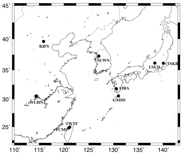
[Table 1.] The names and locations of GPS stations used in this study.
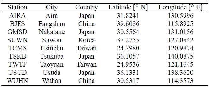
The names and locations of GPS stations used in this study.
The first kinds of mapping functions were suggested by Saastamoinen (1972) and Marini (1972), and continuously developed by Lanyi (1984), Davis et al. (1985) and Ifadis (1986). Then, the Marini mapping function (Marini 1972) was improved into the Herring mapping function (Herring 1992) and the Niell Mapping Function (Niell 1996), which used to be the most widely used one up to recently. NMF was built on radiosonde profiles from the northern hemisphere only, so that latitudedependent biases are largest in high southern latitudes (Boehm et al. 2006a). However, lately developed mapping functions have covered this deficiency by using Numerical Weather Models (NWM) provided by European Centre for Medium-range Weather Forecasts (ECMWF). The representative mapping functions based on NWM are the Vienna Mapping Function (VMF; Boehm & Schuh 2003), the Vienna Mapping Function1 (VMF1; Boehm et al. 2006b), and the Global Mapping Function (GMF; Boehm et al. 2006a).
Some previous researches showed that replacing mapping functions from the NMF to state-ofthe- art mapping functions such as VMF1 and GMF not only affect on tropospheric delay estimates but also influence vertical position estimates. Boehm et al. (2006a) analyzed the height changes by testing NMF, GMF, and VMF1 in GPS analysis, and found that the agreement between VMF1 and GMF is very good, but NMF had the largest difference in south of 45oS, and in the northeastern China and Japan, with station height differences up to 10 mm. As well, Munekane et al. (2008) proved that it is possible to remove annual signals from the vertical GPS time-series by correctly modeling tropospheric delays, and that the precision of height time-series does improve when the latest mapping function was utilized.
In this paper, we analyzed the variation of tropospheric delays and vertical deformations caused by different mapping function in GPS data processing. To quantitatively estimate effects of tropospheric mapping functions, we used nine GPS stations located in the Korean peninsula and surrounding areas in the range of 20oN - 40oN and 110oE - 145oE. We processed the GPS data collected at the selected stations by using GIPSY-OASIS II for four years from January 2005 through December 2008. The nine permanent GPS stations used in this study are listed in Table 1 with their locations denoted in Figure 1.
The three mapping functions tested in this study commonly use the Herring type of continued fraction as shown in Equation (2), and each mapping has a different way of determining its coefficients (Herring 1992). The mapping function
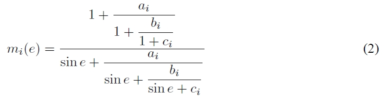
For NMF, VMF1, and GMF, the coefficients
NMF sets its coefficients by applying ray-tracing to nine elevation angles from 3o to 90o on radiosonde data, which had been collected for one year between 1987 and 1988 (Niell 1996). The coefficients are provided only at four latitudes; 15, 30, 45, and 60oN. Thus, for a site not located at those four latitudes, the coefficients should be determined by linear interpolation. The coefficients of the wet mapping function are defined as a constant by latitude, and those of the hydrostatic mapping function are defined as a function of latitude and observation time as follows (Niell 1996):
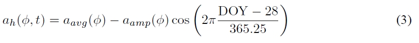
In the Equation (3), φ is the site latitude and Day-of-Year (DOY) is the date based on UT (Universal Time).
The hydrostatic mapping function of NMF needs correction terms to make up for the heightdifference of observation site. Therefore, the hydrostatic mapping function of NMF should be redefinedas Equation (4) with correction terms:

In the equation,
To determine its coefficients, VMF1 uses ray-tracing of NWM instead of radiosonde data. The coefficients

The constant coefficients
VMF1 has a weakness that it has to directly apply ray-tracing by using a NWM in order to calculate the coefficients
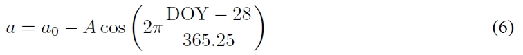
In Equation (6), the coefficient
3. Comparison of Mapping Functions
To analyze the effects on the tropospheric delay and vertical deformations caused by different mapping functions used in GPS data processing, a high-precision GPS data processing program called GIPSY-OASIS II was used (Webb & Zumberge 1993). Except for mapping functions, the same error correction model and processing techniques were applied. In the data processing, the tropospheric delay estimates produced every 10 minutes with GIPSY-OASIS II were converted into daily average values, and daily three-dimensional position estimates were converted into ITRF2005.
In the GPS data processing, a priori values of the hydrostatic and wet delay were set at default ones, and then the remaining Zenith Delay Correction (ZDC) was estimated as a random walk process (Bar-Sever et al. 1998). The Zenith Total Delays (ZTD) is thus the sum of a priori values and ZDC estimates. In this study, we used ZDC estimates to assess the effect of mapping functions on tropospheric delays.
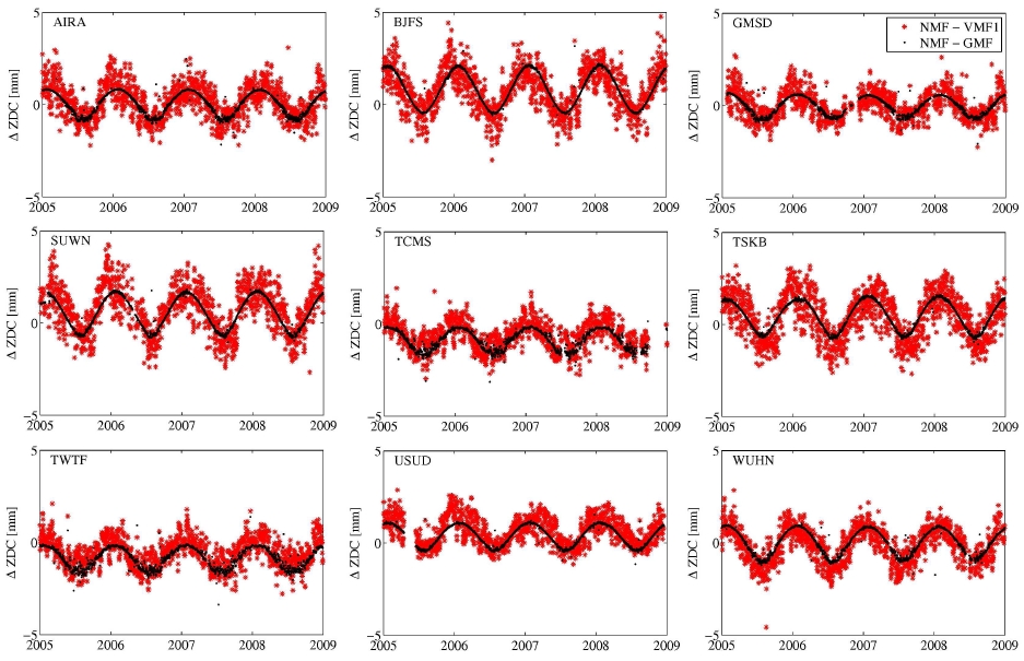
Figure 2 shows the differences of daily ZDC averages at each GPS station. The differences between NMF and VMF1 are marked with red dots and those between NMF and GMF with black ones. In VMF1 and GMF, the effect that the change of mapping functions has on tropospheric delays has a similar bias and seasonal variability compared with NMF. However, the differences in VMF1 have a relatively wide degree of scattering, while those in GMF have a relatively narrow one. Also one can see that the differences of tropospheric delays have maximum values in either February or August.
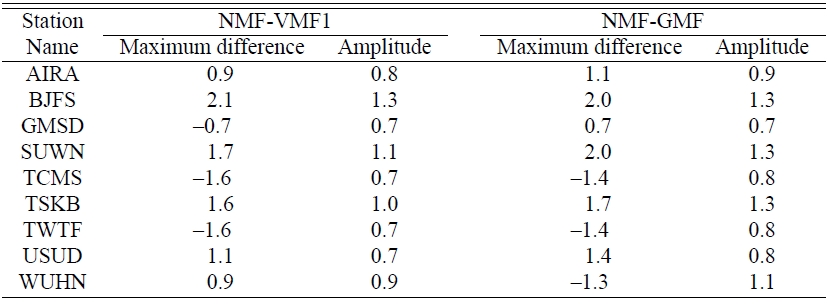
The time series of the differences shown in Figure 2 were curve-fitted with sinusoidal functions and the resulting amplitude is shown in Table 2 along with the maximum differences. The maximum values of differences in Table 2 quantitatively present the maximum changes that VMF1 and GMF have against NMF. The differences in tropospheric delays caused by different mapping functions display the largest difference and amplitude at BJFS and the least at GMSD. However, as mentioned above, the maximum differences in Table 2 are the values smoothed with curve-fitting. Thus even if the maximum difference was 2.1 mm in NMF-VMF1 at BJFS, the largest difference might be up to 5 mm according to Figure 2. In addition, as the differences of tropospheric delay estimates were analyzed as daily average values in this experiment, the effect that the change of mapping functions have on tropospheric delays would be even larger if tropospheric delays are estimated at an interval of 1 hour or 10 minutes.
[Table 2.] The maximum difference and amplitude of the curve-fitted tropospheric delay differences.

The maximum difference and amplitude of the curve-fitted tropospheric delay differences.
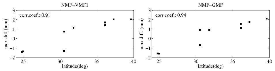
The differences of tropospheric delay estimates are caused because the way that coefficients of NMF, VMF1 and GMF were determined is different from one another. Boehm et al. (2006b) showed that the hydrostatic coefficient
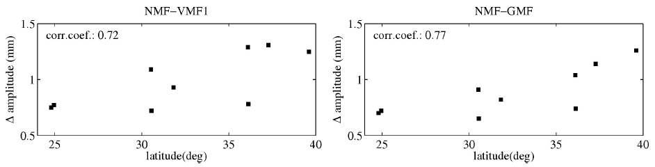
The correlation coefficients of the maximum difference of tropospheric delays and site latitude were larger than 0.9. As illustrated in Figure 3, the differences between NMF and GMF are the least in the area of 30o latitude. The periodicity for the differences of VMF1 and GMF relative to NMF reflects the influence of the season with their magnitude represented in amplitude. As seen in Figure 4, the correlation coefficients between amplitude and the latitude are slightly larger 0.7, which are less than those between the maximum difference and the latitude. Besides, the higher latitude goes, the larger the amplitude gets. Strangely, two GPS stations located at around 30oN and 35oN have less amplitude than those at ∼25oN and they are GMSD and USUD, respectively, located in Japan. Except for those two stations, it is certain that amplitude gets larger as latitude goes higher.
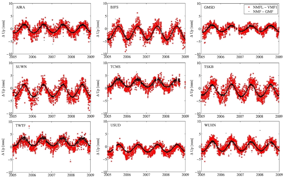
In space geodetic techniques, the precision of the vertical positions has a high correlation with tropospheric delay estimates. MacMillan & Ma (1994) showed that the height error is approximately one-fifth of the tropospheric delay errors at the elevation angle of 5o, and Park et al. (2007) found that the error of vertical crustal deformation and the variation of ZWD had a scale factor of 3.72, depending on the correction of ocean tide loading. To analyze the variations of height estimates by different mapping functions, we used the same GPS data and processing approach as in section 3.1. Figure 5 presents the differences of vertical positions. The differences between NMF and VMF1 are marked with red dots, and those between NMF and GMF with black dots. The height differences by changing mapping functions have the same kinds of annual signals as tropospheric delays, and their magnitudes are almost twice as those of tropospheric delays in the opposite direction.
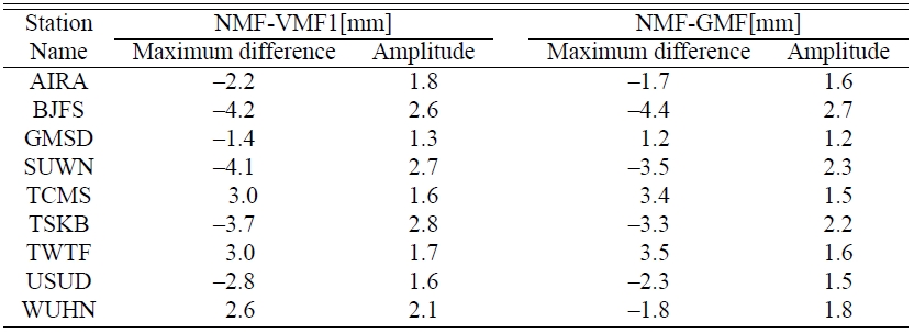
Table 3 lists the maximum difference and amplitude after curve-fitting the time series of the height differences. As shown in the table, the maximum differences and amplitudes by changing mapping functions have the greatest value at BJFS, and the least at GMSD. This is the same result as in tropospheric delays. Two largest height differences were found to be -4.2 mm at BJFS and -4.1 mm at SUWN. However, as illustrated in Figure 5, the height differences can reach up to ≫9 mm in the negative direction at BJFS and SUWN.
[Table 3.] The maximum difference and amplitude of the curve-fitted height differences.

The maximum difference and amplitude of the curve-fitted height differences.
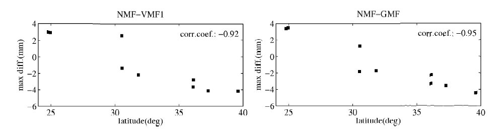
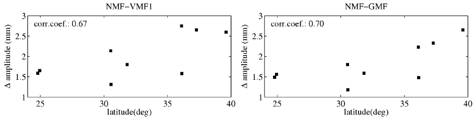
Figures 6 and 7 show the correlation between the height differences and the latitude of the GPS stations. Figure 6 presents the correlation between the maximum difference and latitude, and Figure 7 between amplitude and latitude. The figures show that the maximum differences and amplitudes of the height time series have high correlations with the latitude of the GPS stations. The height differences have the least value around 30oN just as in the tropospheric delay estimates in Section 3.1.
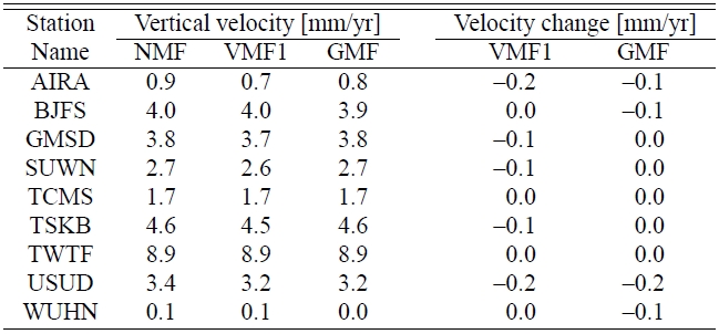
It was anticipated that the vertical coordinate variations due to different mapping functions would be accompanied by the changes in the estimated vertical velocity and their RMS (Root Mean Square) values. Thus, we analyzed the variation of the vertical velocity and RMS by changing mapping functions and assessed their effects. The vertical time-series produced by using NMF, VMF1 and GMF were fitted as a linear regression to estimate the linear velocity and the result is listed in Table 4. In the table, the velocity differences of VMF1 and GMF with respect to the one determined with NMF are also shown. The RMS values of each mapping function and the improvement ratios relative to the NMF are shown in Table 5.
[Table 4.] The vertical velocity change due to different mapping functions.

The vertical velocity change due to different mapping functions.
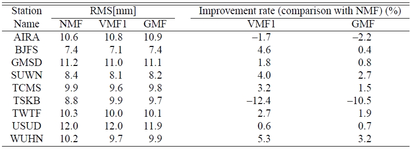
[Table 5.] The variation of vertical velocity and its precision due to mapping functions.

The variation of vertical velocity and its precision due to mapping functions.
As listed in Table 4, vertical velocities showed maximum differences of -0.2 mm/yr at AIRA and USUD, which means that the change of mapping function had little effect on the vertical velocity. From Table 5, we found that RMS or the precision got better at all the GPS stations excluding AIRA and TSKB. For those stations where RMS got lower, VMF1 had more improvement than GMF. One interesting thing to note is that the three sites showing more than 4 % improvement of RMS are located in South Korea and China. And the improvement is less than 2 % or negative for those stations located in Japan. Consequently, it could be hypothesized that the accuracy of the latest mapping functions has a regional or spatial correlation. However, the number of sites used in this study is not large enough to validate this hypothesis. Also further investigation is due for the AIRA and TSKB stations where the vertical precision got worse.
To analyze the effect of mapping functions, nine GPS stations located in 20o - 40oN and 110o - 145oE were selected and their data were processed with the VMF1, GMF, and NMF mapping functions. As a result, the differences of tropospheric delays and vertical coordinates caused by different mapping functions displayed annual signals and showed maximum values in either February or August. Additionally, the maximum difference was observed for the case of VMF1, compared with NMF as reference. The largest difference in the daily average of tropospheric delays was ≫5 mm, and that of vertical positions was ∼9 mm. The differences in tropospheric delay and height estimates had high correlations with the latitude of GPS station, and they had the minimum correlation around 30oN. As well, the correlation between the latitude of GPS stations and the amplitude of curve-fitted differences had a smaller correlation coefficient than that between the latitude of GPS stations and the maximum difference. But the higher latitude goes, the larger amplitude gets excluding two sites. To analyze the effect of the vertical time series induced by different mapping functions, we estimated three different sets of linear velocities at each site. The result shows that the vertical velocity change had a maximum value of -0.2 mm/yr. Therefore, we concluded the change of mapping functions had little influence on the vertical velocity. However, the precision of the vertical time-series was improved almost at all stations.