The unmanned aerial vehicle (UAV) recovery method, especially for an emergency situation, is an important issue in the UAV research community. The reliability and survivability in the case of an unexpected emergency situation, such as global positioning system (GPS) jamming, are critical problems in the operation of UAVs because they are equipped with high-cost devices, such as inertial navigation system (INS), flight control computer (FCC), vision systems, and so on.
In UAV applications, the navigation system can be categorized two types: inertial navigation and referencebased navigation. An INS provides the vehicle's position, velocity, and attitude from a dead-reckoning measurement of the vehicle's acceleration and rotational rate. It is evident that INS outputs are more inaccurate with the passage of time due to the integration process of a dead-reckoning measurement. In other words, INS has a diverging-error characteristic, which renders the vehicle unstable. While GPS gives a vehicle's position accurately, it also offers longterm stability. However, the main drawback is its dependency on satellite signals, which can be easily jammed by some interference.
Nowadays, an INS/GPS integrated system is suggested to increase the accuracy of navigation systems. However, an INS/GPS integrated system also can frequently suffer from GPS jamming. In this case, accurate navigation is impossible due to the diverging-error characteristic of INS. Then, such inaccurate vehicular state information can make a vehicle unstable. At worst, it could be a cause of UAV crash on the ground. In such an emergency situation, the UAV needs to return to its base to save itself without the aid of GPS. This is a critical problem in the operation of UAVs.
Many researchers have considered the UAV recovery method in emergency situations as discussed above. To handle this problem, they have proposed that the UAV immediately land at a nearby, safe region instead of returning to the base. Saripalli et al. (2002) proposes the idea of autonomous helicopter landing using a vision sensor when a UAV is placed in an emergency situation. It assumed that a helicopter can recognize the landing site. Theodore et al. (2006) and Bosch et al. (2006) suggest autonomous UAV landing at an unprepared site using stereo or mono visual sensors. However, they cannot provide a complete solution for UAV recovery. Although a UAV can land at an unprepared site without the aid of GPS, we should know exactly where it has landed to recover it. It is altogether another problem to recover a UAV. For this reason, we suggest a different approach for UAV recovery in this paper. Instead of landing at a nearby, safe region, we consider a method whereby the UAV returns to the base using a dead-reckoning INS without the aid of GPS. As mentioned above, using only INS, it is hard to make a UAV accurately return to its base. Therefore, we suggest a new navigation algorithm in conjunction with SLAM to replace the established navigation method.
Simultaneous localization and mapping (SLAM) (Durrant-Whyte and Bailey, 2006; Gamini Dissanayake et al. 2001) is a popular method for robotics. It is the process by which a robot can build a map of an unknown environment and simultaneously use this map to compute its position. Extensive research on SLAM (Gamini Dissanayake et al. 2001) shows that the error of the map reaches a lower limit, which is a function of the error at the time of the first observation. For these reasons, a SLAM algorithm can help an INSbased navigation system without the aid of GPS to prevent its error of divergence with regard to the vehicle position. Kim and Sukkarieh (2003) applied this method to UAVs, and demonstrated that an airborne SLAM was possible using only vision and INS sensors. Kim and Sukkarieh (2003) furnish the main idea and intuition for our study. We apply the concept of an airborne SLAM algorithm for the UAV recovery method. This can make it possible for a UAV to return to its base accurately. A SLAM algorithm can reduce the vehicular position and map uncertainties when re-observations are made. In a SLAM algorithm, the re-observation process increases the correlation between the map and the vehicle. It is an important and interesting characteristic of SLAM algorithms for mitigating the positional error. Especially in this paper, the proposed method focuses on path planning that maximizes the correlation between landmarks when a SLAM algorithm is used for a supplementary navigation system. The proposed path planning consists of several circular closed paths for using the re-observation process. When a UAV flies along the path proposed by a SLAM algorithm, the errors in the UAV positions are dramatically reduced. In this paper, a SLAM algorithm based on extended Kalman filter (EKF) is formulated. The detailed algorithm is covered in Bailey (2002). For simplicity's sake, planar motion of a blimp-type UAV is considered and pointed-shape landmarks are introduced.
This paper consists of five sections. A general formulation of the problem considered is given in Sec. II. The SLAM algorithm based on EKF for our vehicle model is derived in Section 3. The proposed UAV recovery method, which focuses on path planning for use in the re-observation process, is described in Section 4. In Section 5, the proposed method is demonstrated and evaluated by a number of simulations. The final section concludes the paper.
It is well known that the full SLAM problem of UAVs is complex and difficult to handle. In spite of extensive research activities on SLAM-related problems, a complete solution is not determined as yet. As has been discussed above, this work deals with a new UAV recovery method that is focused on path planning and not a SLAM algorithm itself. Therefore, we introduce some assumptions to avoid a waste of effort. In Section 3, a simplified SLAM algorithm will be formulated under the following assumptions.
1) A 3-DOF model, viz., planar motion of UAVs, is considered.
2) Three-dimensional, pointed-shape landmarks are used.
3) Bearing and range measurements with noise are available.
4) Each landmark has its own ID. In the other words, data association is known.
5) Process and measurement noises are Gaussian.
6) A blimp-type of UAV model is used.
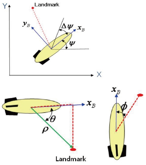
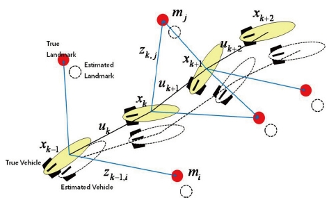
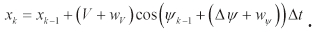
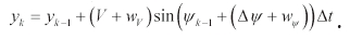
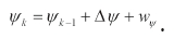
Unlike the case of ground vehicles, the stability of an aerial vehicle is highly dependent on the SLAM algorithm. If the SLAM algorithm is not working well, then an aerial vehicle may crash into the ground because the SLAM algorithm's outputs are highly related to the vehicle's stability. That is why an airborne SLAM is more difficult than other SLAM contexts such as ground robots and cars. To address the stability problem regarding aerial vehicles, a blimp-type model is considered in this paper. Then, three states are needed to describe the motion of the vehicle because a planar motion of UAVs with a certain fixed altitude (100 m) is considered. In this vehicle model, the control inputs consist of the vehicle velocity and vehicle heading angle described in the left of Fig. 1. Each command is denoted by
In the above,
ψ k : The angle at which the vehicle is headed at time k.
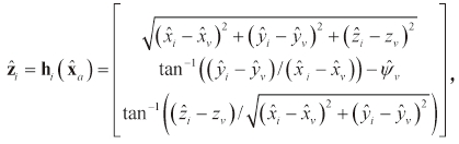
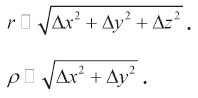
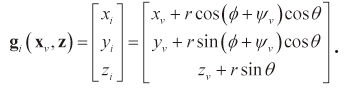
Landmarks are observed by a vehicle from a map in the same coordinate system as that defined in the vehicle model. As already discussed above, three-dimensional, point-shaped landmarks are used in this paper. Landmarks are observed by a sensor, which gives two noisy bearing measurements and a noisy range measurement between the vehicle and an observed landmark. This is shown in the right of Fig. 1. φ represents an azimuth angle measurement and θ denotes the angle of elevation between the vehicle and the landmark. ρ is the range measurement. It is already assumed in this work that these measurements are available. Then, the observation model is formulated as follows:
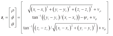
where
xv, yv, zv : The vehicle position. zy is a fixed altitude (100m).
xi, yi, zi : The location of the ith landmark.
vr : The range measurement noise, which is Gaussian noise.
vφ : The azimuth measurement noise, which is Gaussian noise.
vθ : The elevation measurement noise, which is Gaussian noise.
The SLAM process can be described as in Fig. 2. A vehicle starts in an unknown environment and makes a map, which it simultaneously uses for its navigation. The vehicle propagates using an inertial sensor measurement and the vehicle model as discussed in Section 2. When a measurement sensor detects landmarks from the unknown environment, these successive measurements are used to update the vehicle state in terms of the position, velocity, and attitude. Simultaneously, the updated vehicle state is used to update the constructed map.
The above approach is based on the fact that there are statistical correlations between a vehicle position and observed landmarks. These correlations increase when reobservation is made using old landmarks. Therefore, when a vehicle flies along a closed path several times in an unknown environment, errors in the map reach a lower limit, which is a function of the error that existed when the first observation was made. This means that a vehicle can navigate using the SLAM algorithm with reasonable accuracy. The detailed SLAM process is described in Durrant-Whyte and Bailey (2006). In this section, we briefly explain the SLAM process as follows.
The SLAM process,
Step 1: A vehicle located at xk observes two landmarks, mi and mj , at time k.
Step 2: A control input is applied to the vehicle; then, it moves to location xk+1. It re-observes landmark mj ; this causes the estimated vehicle state and map to be updated.
Step 3: Because observed landmarks are correlated with each other, an observation of landmark mj is used to update the previous landmark, mj.
Step 4: New landmarks observed at location xk+1 are linked to the rest of the map, viz., mjand mj .
Step 5: The vehicle proceeds through an environment, and repeats step 1 to 4 to form a map and estimate its state. When re-observations are made, the correlations are increasing. This means that the map precision is increasing.
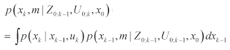
The SLAM problem can be described by probabilistic distributions. It is given below.
n Eq. (5),
xk : The vehicle state at time
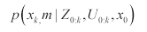
This probability distribution gives the joint posterior density of landmark locations and vehicle states at time
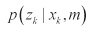
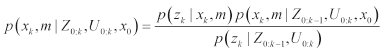
The observation model is defined by a likelihood density function, which describes the probability of making an observation given the vehicle states and landmarks.
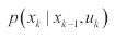
The SLAM algorithm consists of two parts. One part is the time-update step and the other is the measurement-update step. It performs an iterative procedure for computing the joint posterior probability distribution. Detailed information can be found in Durrant-Whyte and Bailey (2006). The SLAM algorithm is briefly described below,
The time update process:
The measurement update process:
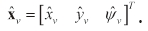
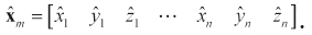
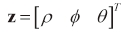
The formulations of SLAM based on EKF for the vehicle model as described in the previous section are presented in this section. These formulations are provided in Bailey (2002). This work considers only two-dimensional equations for a ground vehicle; therefore, we reformulate the threedimensional SLAM equations for our purpose. The vehicle state-vector,
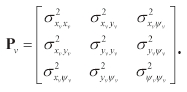
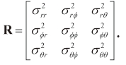
Three-dimensional, pointed-shape landmarks with covariances are defined as below.
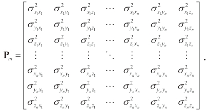
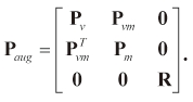
Off-diagonal terms in the above covariance matrix represent correlations between landmarks. When a reobservation process is made, these correlations will increase. SLAM states consist of vehicles and landmark states. These states are constructed by the augmented state vector as shown below.
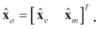
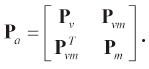
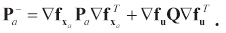
In the above, Pa denotes the error covariance matrix of the SLAM state. In the predictive step, vehicle states are propagated by using the vehicle model and an inertial sensor measurement as described above. The predicted SLAM states, (X^-a) , and the error covariance, Pa- , are given as:
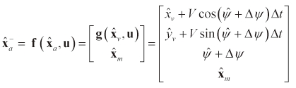
and
In the above,
Q: The control noise covariance matrix.
u: The control inputs, which consist of the velocity,
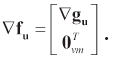
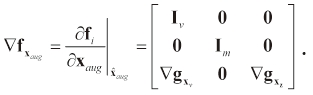
The Jacobian matrices of ∇fxaand ∇fu are defined as:
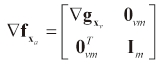
The Jacobian matrices of ∇fxaand ∇fu are defined as:
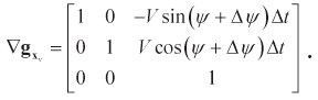
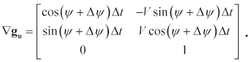
The Jacobian matrices of ∇gxand ∇gu are given as follows.
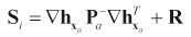
In the update step, the measurements and the error covariance, R, are determined as:
and
The nonlinear relationship between the vehicle state and the observed ith landmark, (xi, ?i, zi) is shown as follows:
where
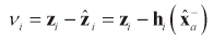
and

In the above, the Jacobian, ∇hx, is given as below.
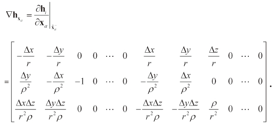
In Eq. (28),
Δx□xi-xv : The relative distance along the x-axis between the vehicle and a landmark.
Δy□?i-?v : The relative distance along the y-axis between the vehicle and a landmark.
Δz□?i-zv : The relative distance along the z-axis between the vehicle and a landmark.
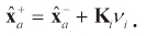
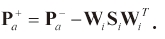
The posterior SLAM estimate is subsequently given by the update equation as follows.
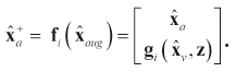
When a new landmark is observed, it should be added to the SLAM state vector. This step is called state augmentation. The method for initializing new landmarks is shown below. A new observation,
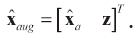
A new observation,
The augmented SLAM state can be estimated by using the following equations.
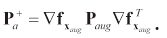
In the above, the Jacobian, ∇fxaug, is given by:
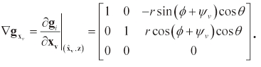
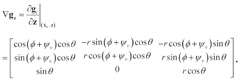
Also, the Jacobian, ∇gx and ∇gx, are determined as follows.
4. The Proposed Method of UAV Recovery
The main idea of the proposed method is based on the ability of the SLAM algorithm, which constrains uncertainties in the vehicle position. Extensive research on SLAM shows that the error in the map reaches a lower limit, which is a function of the error that existed when the first observation was made. In Section V, we will demonstrate how to impact the errors regarding the UAV position and map, when the UAV re-observes already registered old landmarks. This result also was demonstrated by a real flight test in Bailey (2002) and gives a motivation for this work. Note that to reduce the uncertainty in the vehicle position, a re-observation process for old landmarks is recommended. This means that path planning is important to enhance the ability of the SLAM algorithm. Therefore, in this paper, the proposed method focuses on path planning to maximize the correlation between landmarks and minimize errors in the UAV position and map using the EKF-SLAM algorithm.
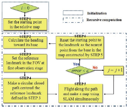
The proposed UAV recovery process is described below. In addition, Fig. 3 provides a flowchart of the process.
STEP 1: Set a starting point in a map.
When a UAV equipped with an INS/GPS integrated navigation system flies in an unknown environment, the GPS is suddenly jammed by some interference. Then, we regard the final GPS position data as the starting point of the map.
STEP 2: Calculate the heading toward the base.
Next, we compute the heading toward the base. It is assumed that the absolute location of the base, (
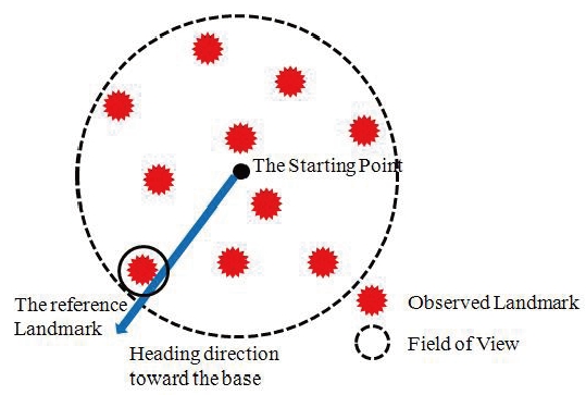
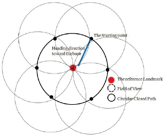
STEP 3: Set the reference landmark in FOV at the first observation.
To maximize correlations between landmarks, a reobservation process is important. To fulfill this requirement, we introduce the reference landmark in the field of view (FOV) when the first observation is made. The reference landmark is defined by the nearest landmark from the base. It should exist in the current FOV. To maximize correlations between landmarks, the reference landmark should exist in FOV at all times when a UAV proceeds through an unknown environment. The underlying idea is to maximize the correlation between landmarks. Figure 4 shows the selection procedure for the reference landmark in FOV when the first observation is made.
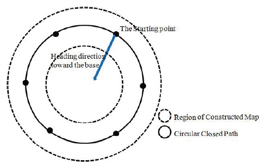
Step 4: Make a circular closed path, which is centered on the reference landmark.
As mentioned in STEP 3, to maximize correlations between landmarks, the reference landmark should be laid on FOV when the UAV flies through an unknown environment. To satisfy this requirement, we suggest a circular closed path as described in Fig. 5. In this case, the radius of the circular closed path is selected as the radius of the maximum FOV.
STEP 5: Flight along the path and the simultaneous generation of a map using SLAM.
The UAV flies along the defined path and simultaneously makes a map using the SLAM algorithm. Section V will show the convergence of the uncertainty of a UAV position when old landmarks are re-observed. When the UAV returns to the starting point as defined in STEP 1, the errors in the UAV position and map are dramatically reduced. To mitigate the positional error by using a re-observation process, at least one rotation of a circular closed path is needed.
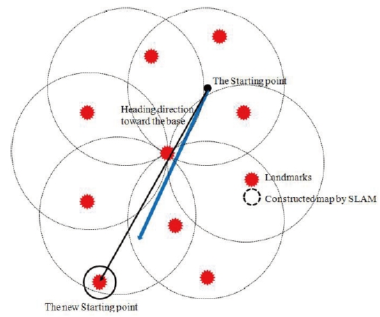
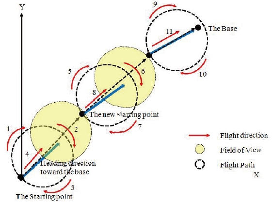
STEP 6: Reset the starting point to the landmark as the nearest point from the base in the map constructed by STEP 5.
Then, the UAV sets the new starting point to the landmark as the nearest point from the base in the map constructed in STEP 5. Thereafter, STEPs 1 through 6 should be repeated. Through the above steps, the UAV can accurately proceed toward the base. This step is explained in Fig. 6. When the new starting point is selected, the map constructed by the previous step is deleted to relieve the computational load, which is generally proportional to the size of the map. Then, we rebuild a new map from the new starting point.
The main advantage of the proposed method is that it can guarantee a bounded positional error without the aid of GPS. However, a certain amount of returning flight distance and time is recommended. Since the flight distance and time are limited by the specification of the power sources installed in the UAV, the proposed method requires a tradeoff between the flight distance and positional accuracy. A trajectory modification is employed as a remedy. To reduce the required flight distance and time, STEPs 3 to 4 should be modified. In this modification, the reference landmark is not needed. Therefore, the radius of the circular closed path does not depend on the reference landmark. This means that the radius of the circular closed path is increased but the correlation between landmarks is decreased. This explanation is described in Fig. 7.
If we use a modified circular closed path, some of recursive steps between 1 through 6 can be eliminated. Then, the total flight distance is reduced. In this modification, the remaining steps are the same except for Steps 3 and 4. Finally, the suggested trajectory is provided in Fig. 8, which describes the proposed recursive steps. When a UAV starts from the position where the GPS is jammed by some interference, it simultaneously builds a sub-map by using the SLAM algorithm along a trajectory, as described in Fig. 8. When the sub-map is constructed, the UAV starts to rebuild a new submap from the new starting point. Then, the UAV flies toward the base by simultaneously using a recursively constructed sub-map.
The proposed method is evaluated and demonstrated by a number of simulations. The considered simulation parameters are listed in Table 1, which specifies the measurement sensor and inertial measurement unit (IMU). As mentioned in the previous section, we assumed that the UAV proceeds at a fixed altitude (100 m is recommended) with an average velocity of 5 m/s in the following simulations.
[Table 1.] Simulation parameters
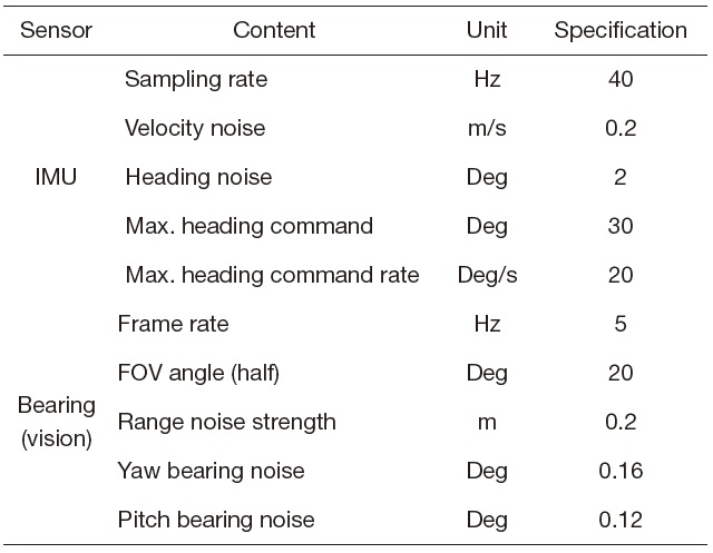
Simulation parameters
The simulation studies consist of three parts. First, the convergence behavior of the UAV position and map using the SLAM algorithm is determined. The estimation accuracy is seen to be highly related to the re-observation process in the SLAM algorithm. The second simulation yields the results of the following scenario. The UAV returns to the base using INS without the aid of GPS when it is placed in an emergency situation especially due to GPS jamming. The third simulation is performed to demonstrate the performance of the proposed UAV recovery method using the SLAM algorithm in the same situation as in Simulation 2.
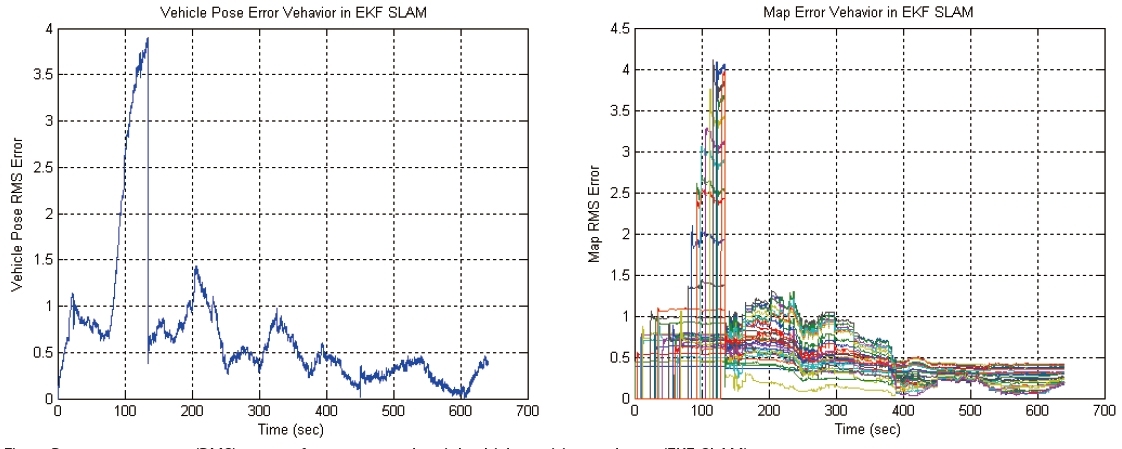
5.1 Simulation 1: The convergence behavior of the map and UAV position
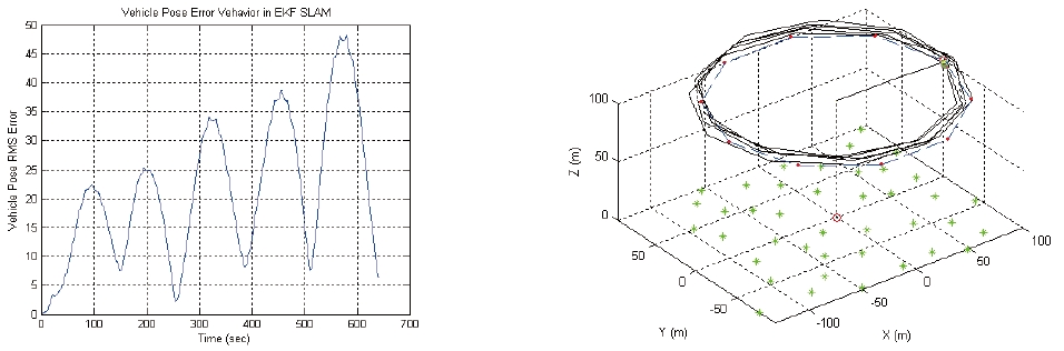
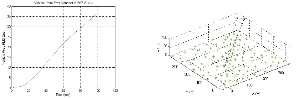
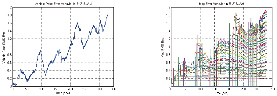
As discussed above, extensive research on SLAM shows that the error in the map reaches a lower limit, which is a function of the error that existed when the first observation was made. This particular simulation is performed to show the converging error behavior regarding a UAV's position and map when the UAV re-observes old landmarks. To measure the error in the estimated UAV and landmark positions, the RMS error is used. It is defined by the square root of the positional error. In this simulation, we consider that a UAV flies along the same circular closed path five times. Simulation results are evaluated by the EKF-SLAM algorithm. Fig. 9 shows the converging error behavior of the UAV position and map while the UAV flies along a circular closed path several times. The RMS errors of the UAV position and map are shown in Fig. 9. When the UAV proceeds along a closed path the first time, the error value is increased. Then, re-observations are made in the second loop. At this moment, the accuracy of estimation is improved. These results reveal why re-observation is important when the SLAM algorithm is performed for UAV navigation systems. Also, the results confirm that the errors in the UAV position and map are limited below a certain level. This fact is a key characteristic of SLAM algorithms and gives the main idea of our work. In addition, to evaluate the SLAM algorithm, we perform the same simulation when the UAV only uses INS data without the aid of GPS. Figure 11 shows an INS diverging error characteristic when the UAV flies along a circular closed path without the support of the SLAM algorithm. In this simulation, the RMS error of the UAV position is increased while the UAV proceeds along a circular closed path due to noisy measurements of the INS output. These results show that the SLAM algorithm can prevent an INS diverging error when the UAV re-observes old landmarks. This is the main idea of this paper for a UAV recovery method without the aid of GPS for an emergency situation.
5.2 Simulation 2: The UAV returns to the base using INS without the aid of GPS
This simulation result also shows an INS diverging error characteristic when the UAV returns to the base from some unknown location without the aid of GPS. In that situation, the UAV proceeds by depending only on a dead-reckoning INS. In this simulation, we set the origin of the map relative to the starting point, which is the place where the GPS signal is jammed by some interference. It is assumed that the UAV's base is located at (353.5, 353.5) m. The initial relative distance between the UAV and the base is 500 m. Then, we consider the problem as how to make the UAV return to the base when it is placed in the discussed emergency situation without the aid of GPS. In this situation, it is assumed that the UAV directly flies along the line from (0, 0) to (353.5, 353.5) m. The results are provided in Fig. 12 as shown below. The left side of Fig. 12 shows the RMS errors of the UAV, while the right side of Fig. 12 gives the flight trajectory of the UAV.
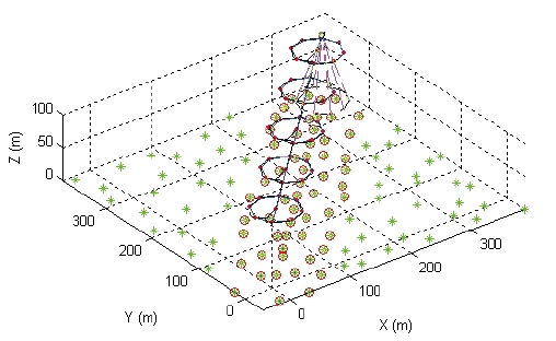
In this simulation, we demonstrate how much the proposed method improves upon the UAV positional error when the UAV is placed in the same situation as mentioned in Simulation 2. To compare with the case of Simulation 2, this simulation is performed under the same conditions. As mentioned in Sec. IV, the proposed method focuses on path planning by maximizing the correlation between landmarks and simultaneously minimizing the errors in the UAV position and map by using the EKF-SLAM algorithm. In Simulation 3, we obtain the behavior of the UAV's positional error while the UAV flies along the proposed path from (0, 0) to (353.5, 353.5) m by using the EKF-SLAM algorithm. The results are given in Figs. 13 and 14. The root mean square error of the UAV position is provided in Fig. 13. It can be easily seen that this value is bounded below 2 m at the base location (final point). In Simulation 2, this value is recorded near 36 m. Compared with Simulation 2, a significant improvement in the estimated UAV position is seen through the proposed method. In Fig. 13, it is also seen that the error in the UAV position is increased slightly according to the time increment. In the recursive step of the proposed method, the new starting point is selected from landmarks in a constructed sub-map, which has a certain extent of landmark positional errors. The proposed method rebuilds a sub-map from the new starting point that contains some error. Therefore, the error is accumulated. This clearly explains why the error in the UAV position is increased at the final position. However, the amount of this error is very small compared to the results of Simulation 2.
Section V provides a simulation result of the proposed UAV recovery method for an emergency situation that is especially for GPS jamming. The proposed method consists of path planning and a SLAM algorithm to reduce the error in the UAV position while the UAV flies along the proposed path. The proposed method is successfully demonstrated by a number of simulations. From the results, the proposed method can be seen to limit a UAV's positional uncertainty while the UAV returns to the base in a discussed emergency situation by depending only on the SLAM algorithm and a dead-reckoning INS for its navigation system. In the final conclusion, the proposed method can make a UAV successfully return to the base in an emergency situation without the aid of GPS.