This article presents a calculation of a reactive flow around an axisymmetric blunt body in the shape of a hemispherecylinder. Experiments for the hypersonic shock tunnel remain a valuable source of information on the physicochemical phenomena that occur in the flow of air surrounding the model. Numerical simulations were used to supplement the theoretical and experimental studies. The simulations were performed by powerful calculators and powerful mathematical tools. In the present work, we implemented a numerical technique to simulate the hypersonic flow around an axisymmetric blunt body. The gas considered is the air in a standard state composed of 21% O2 and 79% N2. The infinite conditions of the flow are those of the atmosphere at a given altitude. In addition, it is necessary to take into account the air under a non-equilibrium state at the exit of a nozzle (Haoui at al., 2001).
Upstream the body, an intense detached shock wave occurred resulting in a very large temperature increase located at the nose of the body just after the shock. For this case, the air starts to dissociate and transforms into a gas composed of five species, O2, N2, NO, O, and N. There are several models that treat chemical kinetics that differ according to the number of chemical reactions. A realistic study must consider all the probable chemical reactions occurring in the flow. For this study, the model with seventeen chemical reactions is selected, 15 dissociation reactions and 2 exchange reactions (Haoui et al., 2001).
Speeds of the reactions employed are based on Arrhenius law. This is in addition to the expression of Landau and Teller (1936) for non-equilibrium of vibration. The time characteristic of vibration is given by the Blackman model (Blackman, 1955). The time characteristic of translation and rotation of molecules are very short in comparison to the time characteristic transition of the flow; however, the time it takes to return to the equilibrium state for these modes is very fast. Note that equilibrium of translation and rotation is carried out in any point of the flow and at any moment. By considering the range of temperatures in which the present study is placed, which is approximately 6,000 K, the phenomena of ionization of the species can be neglected. Similarly, effect of radiation is ignored. The chemical kinetics and the non-equilibrium of vibration are taken into account in the computational domain. The system of nonlinear partial derivative equations which governs this flow are solved by an explicit, unsteady numerical scheme (Goudjo and Desideri, 1989).
The Euler equations for the mixture in non-equilibrium contain mass conservation, momentum and energy equations of the evolution of chemical species (N2, O2, NO, O, N) and the energy of vibration of the molecules. It should be noted that only O2 and N2 species are considered in the non-equilibrium state. The NO molecule is studied under vibrational equilibrium. The time characteristic of vibration of this molecule is lower than that of O2 by two orders of magnitude between the temperatures 3,000 K and 7,000 K (Wray, 1962).
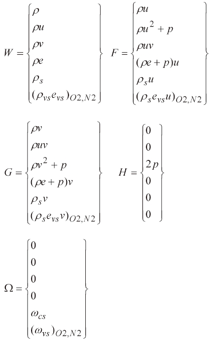
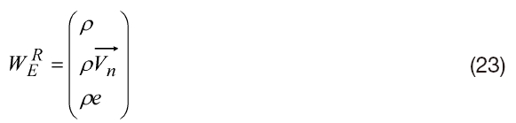
In its vectorial form, the system of equations is written in 3D as follows:
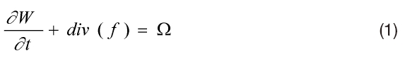
Where:

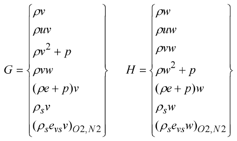
The flux
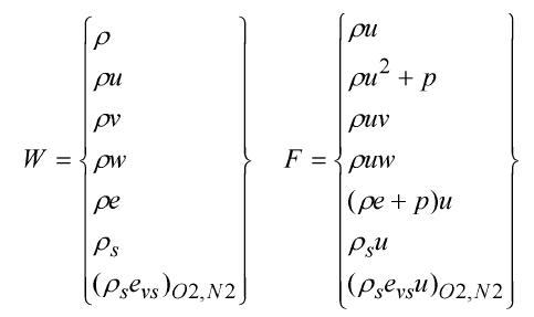
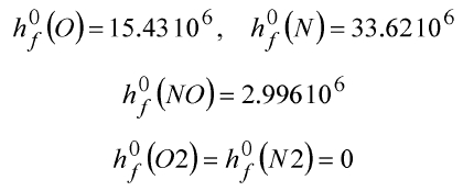
The energy per unit of mass
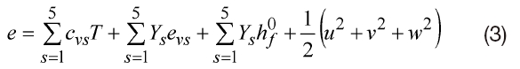
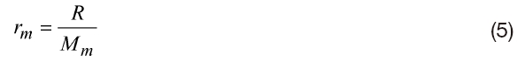
The pressure of the mixture is obtained by the equation of state:
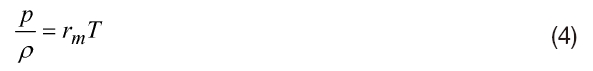
Where
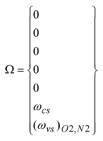
The temperature of the mixture is calculated based on the energy Eq. (3). The source term of the chemical equation of evolution of species
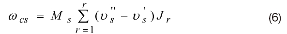
Where:
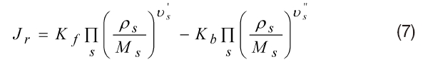
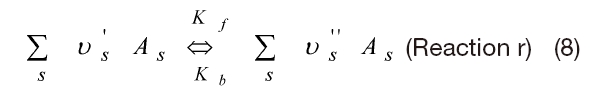
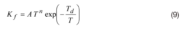
Both forward and backward reaction rates are represented by
The backward reaction rate
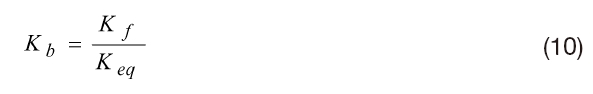
The constants
[Table 1.] Forward constants (Gardiner models)
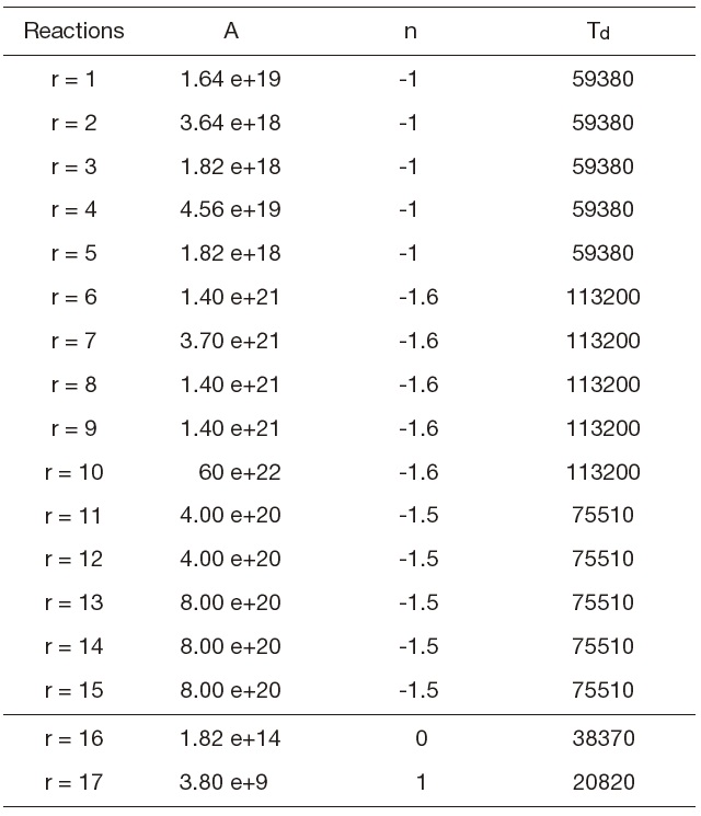
Forward constants (Gardiner models)
[Table 2.] Table 2. Equilibrium constants
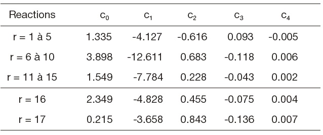
Table 2. Equilibrium constants
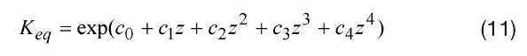
Where
where
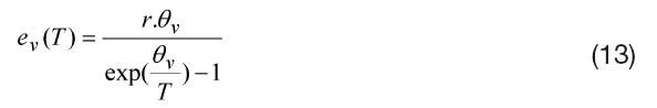
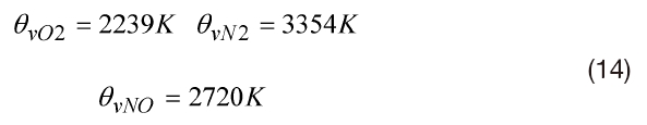
where r is the constant of a particular gas and θv is the temperature characteristic of vibration. It is specified for each molecule. In the present work:

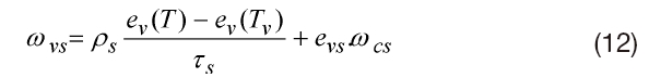
Where
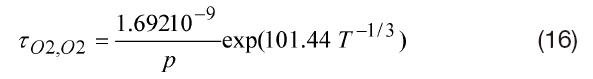
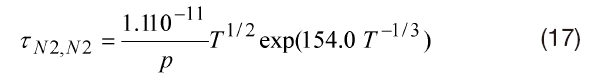
Experiments for binary exchanges, made it possible to evaluate vibrational relaxation time of
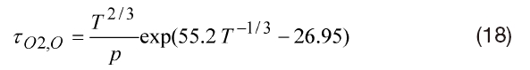
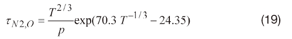
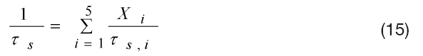
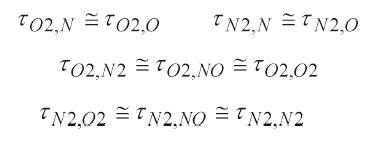
In order to determine the relaxation times, which are not given by the experimental correlations, it is supposed that the relaxation time of a species
The model with 17 reactions is:
O2+M ←→ 2O+M r = 1 to 5
N2+M ←→ 2N+M r = 6 to 10
NO+M ←→ N+O+M r = 11 to 15
N2+O ←→ NO+N r =16
NO+O ←→ O2+N r = 17
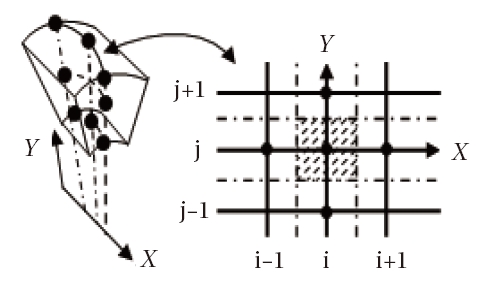
General information is not lost by seeking the solution at the points of an infinitely small domain Fig. 1. A method developed within the Sinus project of the National Institute of Research in Informatics and Automatic (NIRIA) Sophia- Antipolis (Goudjo and Desideri, 1989) makes it possible to pass from 3D to 2D axisymmetric model by using a technique of the disturbance of domain. By taking advantage of this finding, the problem is thus considered as axisymmetric. The system of Eq. (1) can be written as:
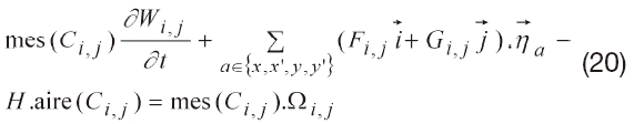
Where mes(
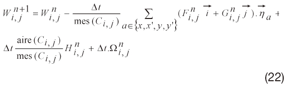
The present numerical method is based on an explicit approach in time and space. The step of time △t is as follows:
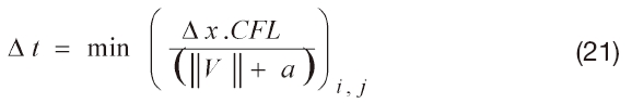
The Courant, Friedrich, Lewis (CFL) is a stability factor.
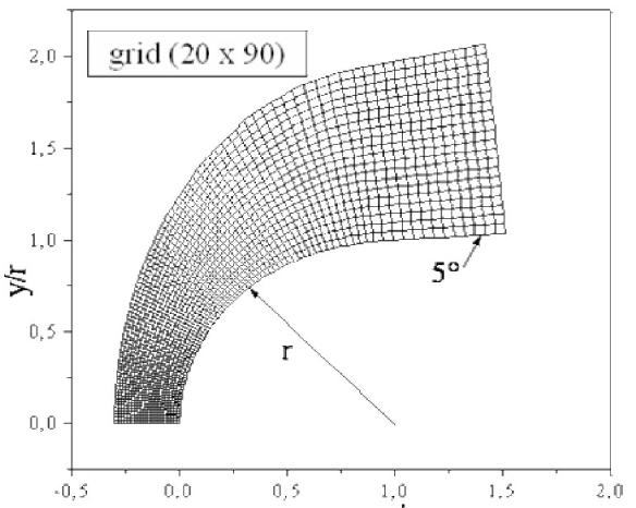
The choice of the grid plays an important role in determining the convergence of the calculations. Therefore, it is indeed advisable to have sufficiently refined meshes at the places where the gradients of the flow parameters are significantly large, as observed in front of the nose of the obstacle.
In this study, the decomposition of Van-Leer (1982) is selected, namely a decomposition of flow in two parts,
The vector
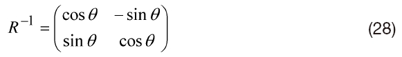
where is obtained from , via the rotation R, in the following way:
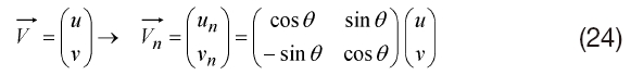
where:
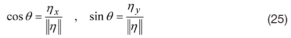

The overall transformation R is
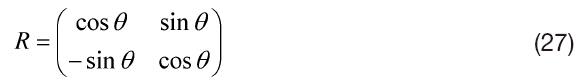
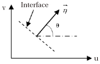
Moreover, at each interface (
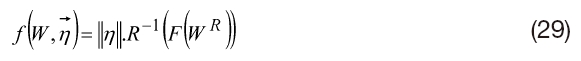
This property makes it possible to use only one component (
The expressions of
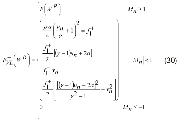
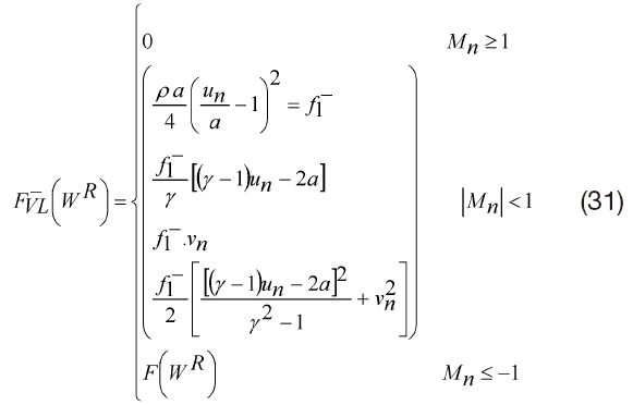
Where ,
On the line of entrance, the parameters
Because flow is not viscous, a slip condition is applied to the wall. At any point,

where is the normal to the wall.
6.3 Axis of Symmetry
In any point

At the exit of the computational domain, which is downstream of the body, the flow is supersonic; the exit values of the flow filed parameters are extrapolated from the interior values.
7. Results and Interpretations
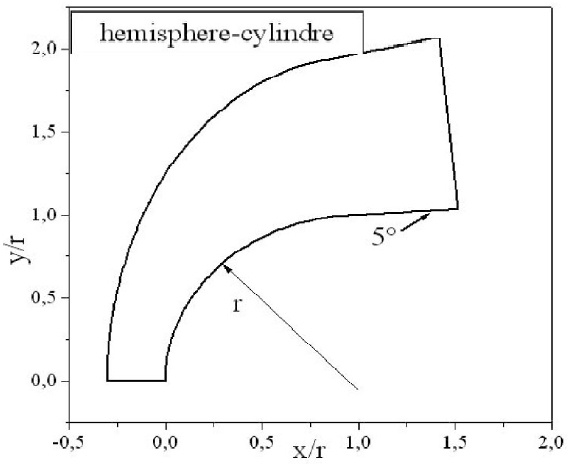
The body employed for the numerical simulations is a hemisphere followed by a cylinder with a 5o conical angle, as depicted in Fig. 3. The grid used in calculations is composed of 40 × 180 nodes. For illustration purposes, an example of grid with the dimensions 20 × 90 is presented in Fig. 4. The composition of the air of the upstream the flow is taken equal to 21%
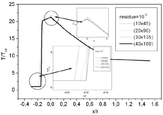
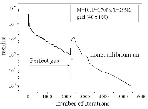
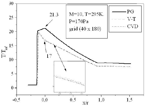
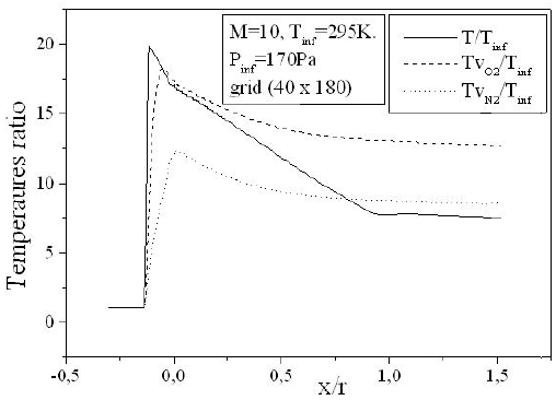
For a flow neglecting the effects of thermo-chemistry, the mass fractions of the chemical species and the energy of vibration are supposedly fixed. The residue of the relative variation of the density is about 10-5. There is no change in the findings for lower tolerance; Fig. 6 shows the variation of the residue according to the iterations count for a grid of 40 × 180 nodes. Figure 7 illustrates the variation of the temperature along the axis of symmetry until reaching a stagnation point, and then along the surface of the body. The difference between the cases of a perfect gas (PG), a nonequilibrium flow without coupling (V-T) and with coupling vibration-dissociation (CVD) according to the Park model (Park, 1989) while replacing the temperaturet
Temperatures obtained in the case of the reactive flow are lower than those of PG. At the stagnation point for example, the ratio of the temperature
Figure 8 depicts the variation of the temperature of vibration of
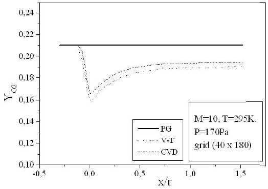
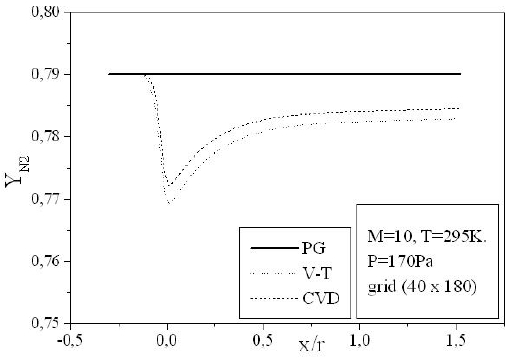
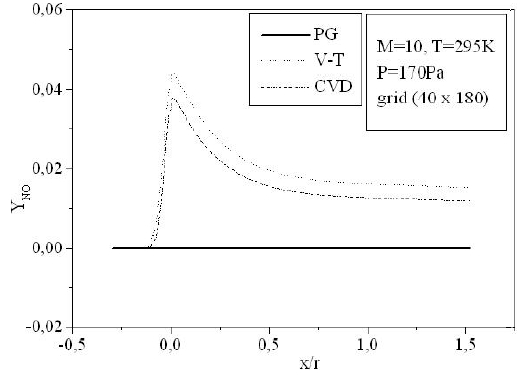
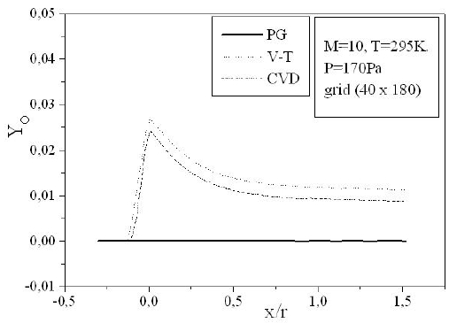
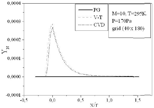
Figures 9-13 illustrate the evolution of the mass fraction of the chemical species constituting the mixture of air. It is noticed that the dissociation of
The mass fraction of the chemical species becomes frozen downstream where
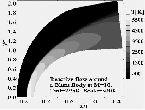
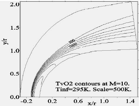
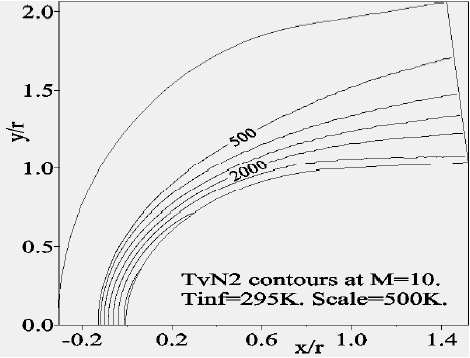
Concerning the flow far from the wall, we presented the Mach-contours around the body in Fig. 14 where the shock wave detachment is visible in front of the nose of the body. The position of the detachment shock does not vary too much compared to the case without chemistry. For the nonequilibrium case, the position of the shock is at 0.135 times the radius in contrast to the case without chemistry (0.150 times the radius). Figure 15 shows the temperature-contours around the body. At the stagnation point the temperature is 5,015 K, whereas just after the shock it increases to 5,870 K; the difference is absorbed by the dissociation of the molecules. In addition, Figs. 16 and 17 depict the temperature-contours of vibration of
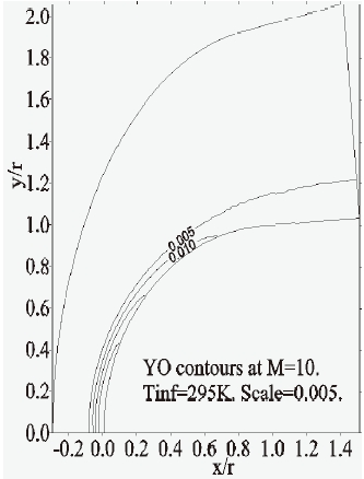
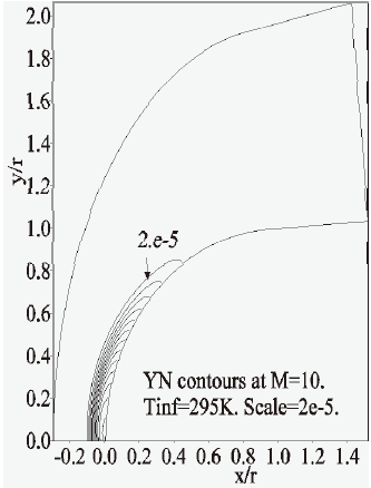
Furthermore, the concentration-contours of
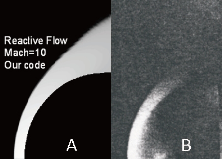
Due to the lack of experimental values in the literature, our results were compared with a real photograph of the same flow (Nagamatsu, 1959), Fig. 20. We can observe the position of the detached shock wave and the thickness of the reactive flow between the shock and the body.
The numerical simulation of flows around blunt bodies at high temperatures provided satisfactory results from a numerical and a physical point of view. With high degree of accuracy requirements, computational convergence is achieved and the physical phenomena considered are visible after the detached shock wave and around the blunt body. The choice of the kinetic model for this type of flows is interesting. The model with 17 reactions proves to be more realistic since it considers all the possible collisions between molecules and atoms of the mixture of air. After the shock, the air is in a state of non-equilibrium, and a frozen state is obtained after the stagnation point, from