The pursuit-evasion game is a kind of differential game demonstrated by Isaacs (1967). It is an important class of two-player zero-sum differential games with perfect information and is useful in military applications, especially in missile guidance applications. In the game, the pursuer and the evader try to minimize and maximize the intercept time or the miss-distance as a payoff function. Among previous studies, Guelman et al. (1988) studied a simple case of pursuit-evasion game that can be solved without addressing a two-point boundary value problem. Breitner et al. (1993) proved that a multiple shooting method is able to precisely solve practical pursuit-evasion games subject to state constraints. In addition to these studies, a variety of parameter optimization methods such as those described in (Hargraves and Paris, 1987) can be extended to solve realistic pursuit-evasion games. In this study, we propose a direct method for solving pursuit-evasion games (Tahk et al., 1998a, b).
We first summarize the algorithm proposed in (Tahk et al., 1998a, b) for the reader's convenience. The algorithm is a direct method based on discretization of control inputs for solving pursuit-evasion games for which the intercept time is the payoff function of the game. Every iteration of the algorithm has two features: update and correction. The update step improves the evader's control to maximize the intercept time, and modifies the pursuer's control to satisfy the terminal condition. After applying the update step several times, the correction step is used to minimize the pursuer's flight time.
Note that the solution of the pursuit-evasion game can be used for guidance of the pursuer and the evader if the solution is obtained in real time. For this purpose, the iteration number of the solver is limited to reduce the computation time, at the cost of solution accuracy (Kim et al., 2006). In this study, the work of Kim et al. (2006) was refined for better numerical efficiency. Also, the capture set of the proposed guidance method is compared with that of proportional navigation to confirm that the proposed differential game guidance laws provide a smaller no-escape envelope.
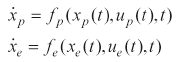
The problem is a two-dimensional pursuit-evasion game with the final time as a payoff function. The dynamics of the pursuer and the evader are expressed as follows:
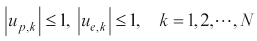
The admissible control inputs

Our pursuit-evasion problem is written as
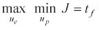
subject to the constraints in Eq. (2) and the final constraint,
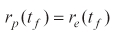
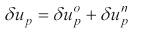
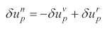
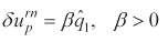
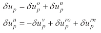
To develop a numerical algorithm, we used a direct approach based on parameterization of the control inputs. The control inputs of both players are separated into the following form:
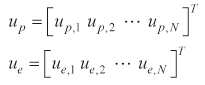
where
The solution technique proposed in (Tahk et al., 1998b) is composed of two procedures: update and correction. The update procedure determines δ
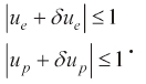
We assume that a capture within a finite time is guaranteed. Any perturbations of both players' control input, δ
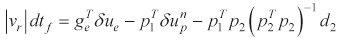
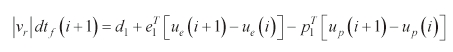
The capture condition is expressed as
where
and
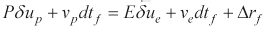
Then, Eq. (8) can be written as
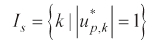
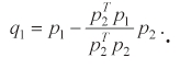
Let

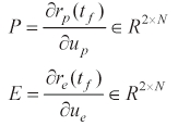
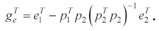
Now,
where
If δ
where δ
where
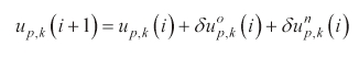
The evader's control input is then updated as follows:
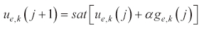
where j denotes the iteration number, and subscript k is kth element of the separated evader's control variables.
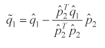
When the deviation of
where δ
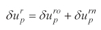
where δ
For minimizing (수식삽입), we find the δ
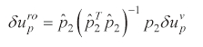
After calculating δ
Once
In Eqs. 22) and (23),
2.2 Step 2 (correction algorithm)
In step 1, the pursuer's control input is determined to satisfy the capture condition, and
Assume that the pursuer's control input is subject to variation, but the evader's control input is fixed; that is, δ
where
The purs
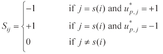
Then, let
Hence, the Kuhn-Tucker condition is written as
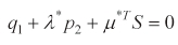
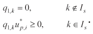
where mk > 0 for all . We also derive the following necessary conditions for optimality:
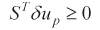
For the correction procedure, we set dδ
We choose d
to reduce
If there is any violation of the control input constraint, we use the
3. Constructing the Proposed Guidance Law
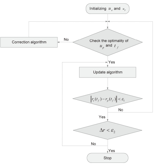
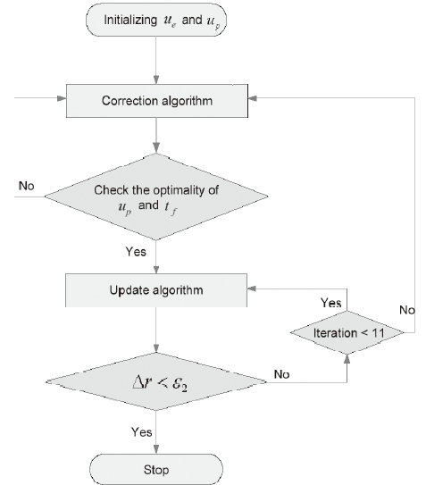
In this section, we explain the method we used to construct the guidance law proposed in (Kim et al., 2006). The algorithm introduced in the preceding section consists of two steps. This algorithm initializes both players' control inputs, and then checks the optimality conditions. If the pursuer's control input and final time do not satisfy the optimality conditions, step 2 is performed; otherwise, step 1 is executed. The evader tries to maximize the final time or to avoid capture by the pursuer, and the pursuer tries to intercept the evader. After performing step 1, we examine whether a difference in the positions of the players at the final time is within the error bound. If it is within the error bound, a variation of the evader's position at the final time is examined. If the variation is within the error bound, the algorithm is terminated and gives optimal trajectories. Otherwise, step 1 is repeated. If the difference in the positions of the players at the final time is not within the error bound, the optimality conditions of the pursuer's control input and the final time are checked again.
The initializations of both players' control inputs are the same as the algorithm proposed in (Tahk et al., 1998a, b). In this case, the algorithm is started with step 2. At the proposed algorithm, step 2 is executed when a violation of the optimality condition has occurred and step 1 is repeated when a variation of the evader's position at the final time is not within the error bound. To construct a guidance law, this procedure is changed to execute step 2 once and step 1 ten times. The dynamics of both players are integrated with specific integration time interval δ
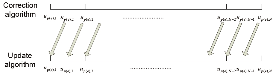
With integration, this modified algorithm changes control inputs. First, control input elements of both players are got rid of the control input sets after an integration and the others are replaced previous elements of each control inputs. The reason is that the first control input elements of the pursuer and the evader are used during integration, and both players' positions are updated by integration. By reason of integration with δ
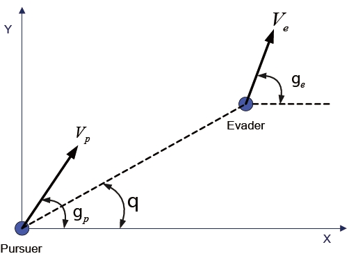
The differential game guidance law proposed in (Kim et al., 2006) wasapplied to the planar pursuit-evasion game problem illustrated in Fig. 4. The equations of motion of the evader are described as
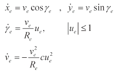
In these equations,
The equations of motion of the pursuer, which are analogous to those of the evader, are as follows:
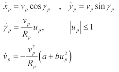
where
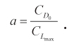
The constant

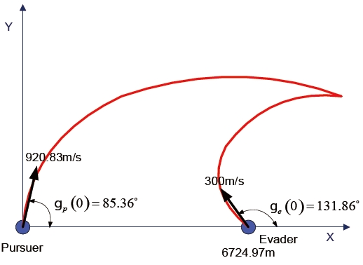
The engagement scenario for the numerical example is shown in Fig. 5. The evader is initially 6,724.97 m apart from the pursuer along the x-axis, and moves with
The differential game guidance law parameters were chosen as
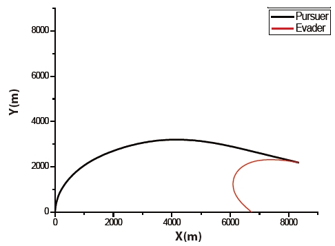
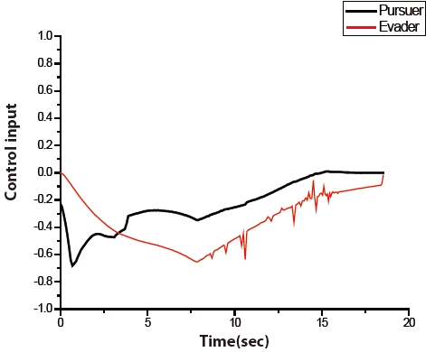
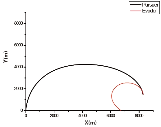
The trajectories of the pursuer and the evader are shown in Fig. 6. The pursuer intercepts the evader at 18.565769 seconds. The time histories of the control input of both players are illustrated in Fig. 7. The figure shows that an initial control input of the evader is a zero. The figure also shows that the control inputs of both players are constrained by Eq. (2).
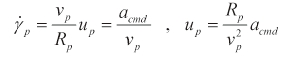
To compare the performance of the differential game guidance law with other guidance laws, proportional navigation guidance (PNG) was adopted as a guidance law of the pursuer. In spite of using PNG, we assumed that the evader knows the maneuvers of the pursuer which are optimal. In this case, the pursuer's control inputs are calculated from
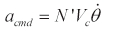
where
It is also constrained by the first expression in Eq. (2). Using PNG as a guidance law, the termination condition is replaced by the miss distance. If the miss distance is smaller than 1 m, we believe that the purs
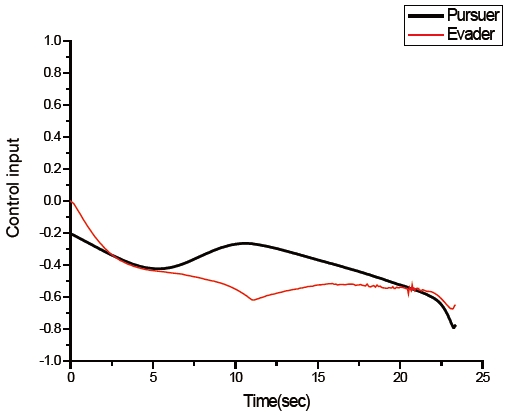
Trajectories of the pursuer using PNG as a guidance law, and of the evader, are given in Fig. 8. The pursuer captured the evader at 23.339497 seconds. Time histories of both control inputs are shown in Fig. 9, and are similar to Fig. 7. The pursuer's initial control input is a few different between the differential game guidance and PNG. This is because a control input of the pursuer using the proposed guidance law is initialized by PNG, and then it is improved by step 2.
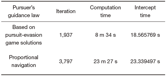
Table 1 is a summary of the simulation results. The intercept time of the differential game guidance law is shorter than the time using PNG. In the case of using PNG, a computation time is approximately three times longer than that using pursuit-evasion game solution. The number of iterations needed to capture the evader is nearly two times greater than that of the proposed guidance law.
[Table 1.] Summary of simulation results

Summary of simulation results
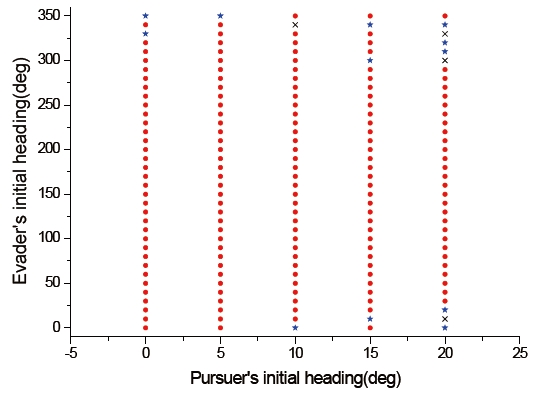
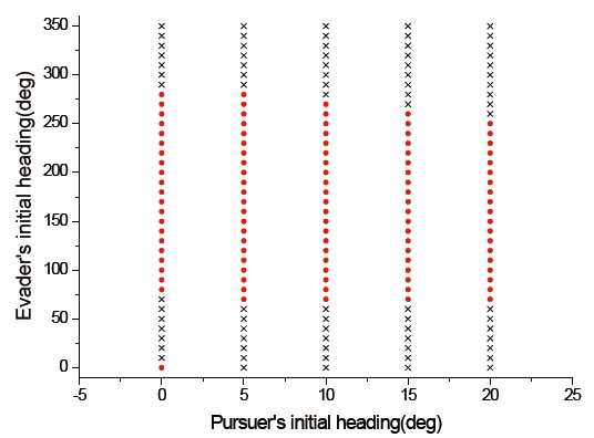
To compare the interception performance of both methods, which are both players using the differential game guidance law and the pursuer using PNG, the capture set was calculated. For simplicity, we considered only the initial condition for the previous example except that the initial flight path angles of the pursuer and the evader varied from 0° to 20° and from 0° to 350°, respectively. The reason why we selected the initial flight path angle ranges of the pursuer is that seeker's gimbals used typical guided missiles adopt lock-on type. The conventional field of view of a seeker is limited from 2° to 5°, but the field of view of seeker-adopted lock-on type gimbals is larger than 15°. The field of view of gimbaled seekers, however, is not much larger than 15°. Thus, the initial flight path angle ranges of the pursuer were chosen as 0° to 20°.
Figures 10 and 11 show the capture sets of the proposed guidance law, and the case using PNG as a guidance law of the pursuer. In these figures, the initial conditions marked with (특수문자) are those for which the pursuer can capture the evader within a finite time. The other symbols indicate the termination of the program without a capture. In Fig. 10, the symbol ★ indicates a circumstance for which the pursuer cannot capture the evader under the termination condition of the differential game guidance law, but is able to intercept the evader under the termination condition when using PNG as a guidance law of the pursuer. The symbol × implies that the pursuer is not able to intercept the evader under both termination conditions. In Fig. 11, the symbol × indicates that the miss distance is larger than 1 meter, so interception by the pursuer does not occur. From Figs. 10 and 11, we know that the capture set of the proposed guidance law is larger than one using PNG as a guidance law of the pursuer.
We carried out a performance analysis of the proposed guidance law based on pursuit-evasion game solutions that were sought by the pursuit-evasion game solver. The derivation of the proposed pursuit-evasion game solver was described, and construction of the proposed guidance law was explained in detail. The guidance law proposed in (Kim et al., 2006) consists of two procedures, update and correction, called step 1 and step 2. Control inputs of the pursuer and the evader were
initialized in the differential game guidance law, and then improved by step 1 and 2. Step 2 executes first that this procedure provides a way to optimize the pursuer trajectory when it deviates excessively from the optimal trajectory. Then, the dynamics of both players were integrated with a specific time interval. Step 1 performs that control inputs of the evader were updated to maximize the increment in the capture time, while the pursuer tried to minimize it. This procedure iterated until satisfying the termination condition. The differential game guidance law was applied to solve a numerical example. For a comparison of the interception performance, PNG was adopted to a guidance law of the pursuer. Simulation results of the engagement scenario were tabulated for each case--the differential game guidance law, and using PNG as the guidance law of the pursuer. Capture sets of both cases were calculated for performance analysis. Based on our numerical example simulation results, we know that the differential game guidance law provided a smaller no-escape envelop than PNG.