The ever-increasing need for more network capacity requires high-performance and high-capacity optical fiber communication systems [1]. A key technique to operate and maintain high-capacity optical networks is cost-effective performance monitoring. Performance monitoring in optical fiber communication systems include (1) monitoring of basic optical parameters (wavelength, power, and optical signal-to-noise ratio) [2-4], (2) dispersion parameters (chromatic dispersion and polarization-mode dispersion (PMD)) [5-10], and (3) bit-level performance parameters (eye opening, Q-factor, and bit-error rate (BER)) [11-20]. Among the above, BER monitoring is the ultimate goal of performance monitoring in all digital communication systems as well as optical fiber communication systems. A BER monitoring technique, enabled by advanced electronic technology, can be used in various fields including the monitoring part of dynamic compensators such as a PMD compensator [20] or a chromatic dispersion compensator [21]. In fact, BER monitoring is more effective than chromatic dispersion monitoring or PMD monitoring for the optimal compensation in the real nonlinear transmission case.

Another issue which must be considered together with BER monitoring is the decision threshold optimization [22]. The level of decision threshold at the receiver is required to be the optimal value to get the best BER. In many optical transmission systems, the level of decision threshold is just set on the averaged DC level of the received signal without any further consideration. However, according to earlier reports, adaptive decision threshold optimization can give a gain of more than 2 dB [23, 24].

In this paper, we analyze a pseudo-error counting schemeand propose an algorithm to achieve both BER monitoringand adaptive decision threshold optimization. To verify theproposed algorithm, we conduct computer simulations inboth Gaussian and non-Gaussian distribution cases.

The scheme of pseudo-error counting has been proposed earlier to estimate BER [15-17]. However, to our knowledge, the earlier researchers have not analyzed this scheme clearly and have not presented a related algorithm. In this paper, we introduce a simpler explanation of the principle of pseudoerror counting and propose an algorithm to estimate BER and optimize the level of decision threshold.

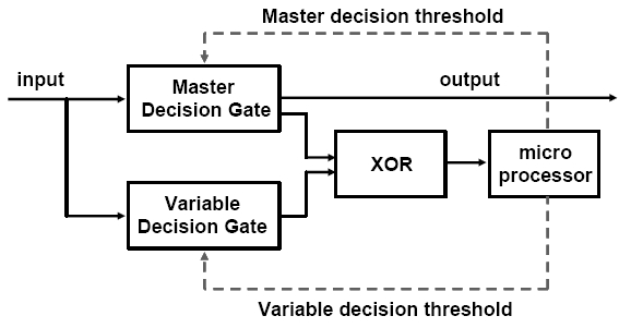
The scheme of pseudo-error counting is shown in Fig. 1 [25, 26]. The master decision gate is for communication and the variable decision gate is for BER monitoring and adaptive decision threshold optimization. Thus the master decision threshold is the main decision threshold required to be optimized. The variable decision threshold is the secondary decision threshold used to obtain the pseudo error. The pseudo error is generated by the decision difference between the two decision thresholds; one is decided by the master decision threshold and the other is decided by the variable decision threshold. The exclusive OR (XOR) gate generates '1' when the outputs of the two decision gates are different. The micro processor counts the total number of pseudo errors and controls the master and variable decision threshold.

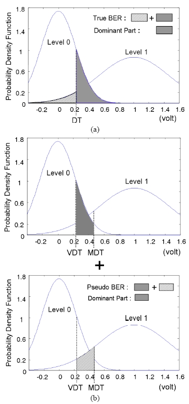
Fig. 2 illustrates the probability density function (or amplitude histogram) of the optical signal and the areas of (a) the true BER and (b) the pseudo BER counted in the micro processor. Adding the hatched area and the shaded area in Fig. 2 makes the total quantities of (a) the true BER and (b) the pseudo BER, respectively. Although the exact values of the true BER and the pseudo BER are different, the dominant parts of the two BERs become similar especially when the variable decision threshold (VDT) is far enough apart from the master decision threshold (MDT).

In the pseudo-error counting scheme, assuming a Gaussianapproximation, the true BER of the received signal and thepseudo BER counted in micro processor are given by

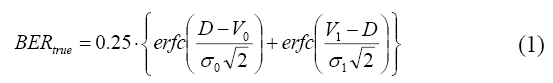
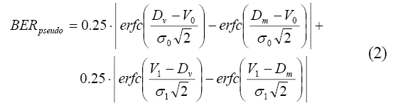
where V₀ and V₁ are the voltage of level 0 and 1, σ₀ and σ₁ are the standard deviation of the noise imposed on level 0 and 1, D is the decision threshold, and D_m and D_v are the master and variable decision thresholds, respectively. Note that the true BER cannot be obtained at the receiver because the original bit stream is not known at the receiver. However, the pseudo BER can be obtained at the receiver using the pseudo-error counting scheme shown in Fig. 1.

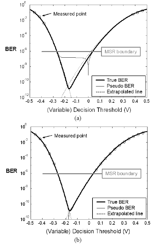
Fig. 3 (a) shows the true BER and the pseudo BER as a function of (variable) decision threshold when the master decision threshold is set to an initial value of 0 V, while the optimum value is -0.17 V. We assumed V₀ = -0.5 V, V₁ = 0.5 V, and the typical noise value of σ₁ ？ 2σ₀. We assumed a Gaussian amplitude histogram. As shown in Fig. 3 (a), the pseudo BER curve itself is different from the true BER curve. However, if the master decision threshold is shifted near to the optimal value, the pseudo BER curve become similar to the true BER curve except a singular point at the master decision threshold, as shown in Fig. 3 (b). Therefore, we can estimate the minimal true BER and the optimum decision threshold by using extrapolation after measuring some points on the pseudo BER curve.

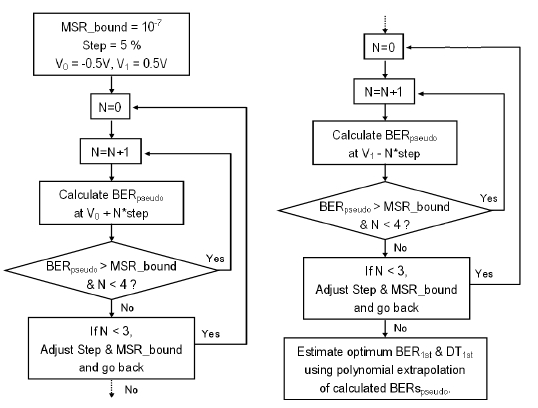
We propose a control algorithm consisting of two steps based on the pseudo-error counting scheme to estimate the optimal decision threshold and BER. The purpose of the first step is shifting the master decision threshold near to the optimal value quickly. Changing the variable decision threshold, three or four points of the pseudo BER are measured and then the optimal decision threshold and the minimal BER are estimated by quadratic extrapolation as shown in Fig. 3 (a). Pseudo BER is measured by counting 100 errors at each point, since it is necessary to count 50~100 errors to get a reliable BER value [27]. There can be small errors when estimating the optimal decision threshold and BER in the first step. After the first step, the master decision threshold is shifted to the estimated optimal decision threshold obtained in the first step. The detail control algorithm for the first step is shown in Fig. 4.

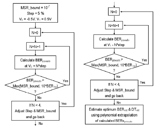
The goal of the second step is to estimate the precise value of the optimal decision threshold and BER. In the second step, several points of the pseudo BER are measured down to the 'Measure (MSR) boundary' we have decided or to 10 times of the estimated BER (BER1st) obtained at the first step. Then, the optimal decision threshold and BER are estimated by polynomial extrapolation, as shown in Fig. 3 (b). The concept of 'Measure boundary' was made to reduce the computing time since it requires a lot of waiting time to count 100 errors in a low value of BER. The detail control algorithm for the second step is shown in Fig. 5. Even after the second step, more iteration similar to the second step can be used to obtain more accurate values. It depends on the required processing time of the system.

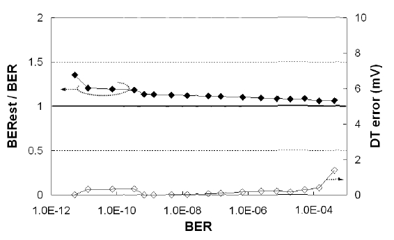
To verify the proposed algorithm, we conducted computer simulations for the ideal Gaussian distribution case, as shown in Fig. 2. All the results in this section are the simulation results after the second step with a measure boundary of 10^-7. Fig. 6 shows the errors of the estimated optimal decision threshold and BER. The BER errors are expressed as the ratio of the estimated BER to the true BER, thus ‘1’ is the perfect value for the BER errors in the graph. The decision threshold (DT) errors are expressed in mV when the 0-1 level difference is 1 V. The results in Fig. 6 show that BER and the optimum decision threshold can be estimated with the errors of < 20% and < 2 mV to the range of ~10^-10 BER, respectively.

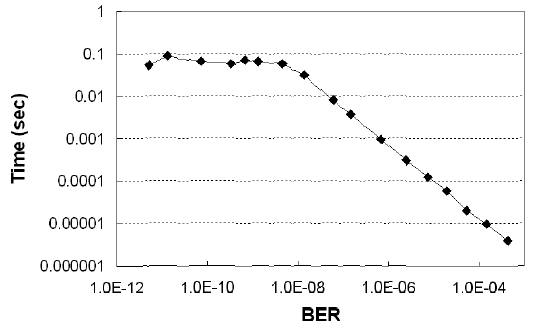
Fig. 7 shows the required processing time by the end of the second step. We summed up the time of the two steps spent on counting 100 errors at each pseudo BER point. Thus the required processing time is not dependent on the performance of the hardware; it is the required theoretical time limit to obtain a reliable BER value. In Fig. 7, the required processing time is less than 0.1 s to the range of ~10^-12 BER. In this calculation, we assumed 40-Gb/s optical transmission system.

The results of this section demonstrate that the proposed algorithm is efficient enough to monitor BER and the optimal decision threshold in a Gaussian distribution case.

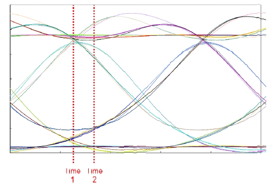
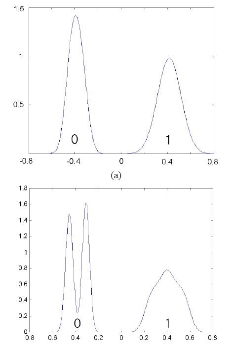
To verify the proposed algorithm in the real transmission case, we conducted computer simulations for the case of non- Gaussian amplitude histogram. Fig. 8 shows an eye diagram of a dispersed optical signal by chromatic dispersion. The amplitude histograms at Time 1 and Time 2 in Fig. 8 are shown in Fig. 9. The amplitude histogram at Time 1 (Fig. 9 (a)) is similar to the Gaussian distribution case. Thus we are not interested in the case of Time 1 in this section. We are interested in the case of Time 2 (Fig. 9 (b)) where the amplitude histogram of level 0 is split by dispersion and that of level 1 is distorted by dispersion.

In this section, an additional iteration after the second step is used to obtain more accurate values. Thus the simulation results in this section are with an additional iteration after the second step, in the case of Fig. 9 (b). A measure boundary of 10^-7 is used in the simulation. In the additional iteration, the optimal decision threshold and the minimal BER is estimated by quadratic extrapolation with the last three pseudo-BER points nearest to the optimum value.

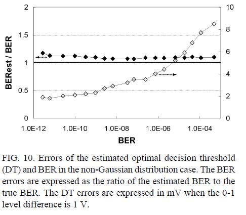
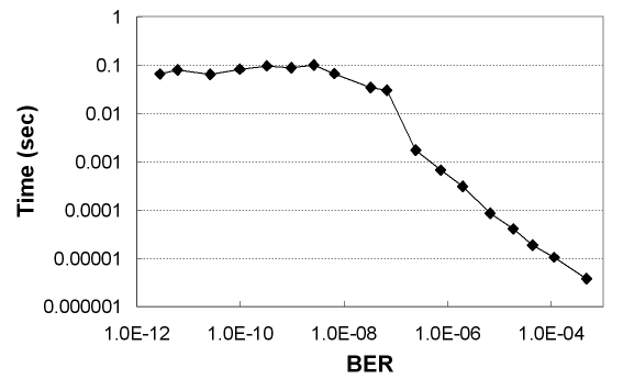
The errors of the estimated optimal decision threshold and BER are shown in Fig. 10. In the non-Gaussian distribution case, the mathematical expression of (1) and (2) cannot be used. Instead, we can obtain the value of the true BER and the pseudo BER by numerically calculating the area of the hatched and shaded areas, the same concept as in Fig. 2, directly from the non-Gaussian distribution. The BER errors are expressed as the ratio of the estimated BER to the true BER. The decision threshold (DT) errors are expressed in mV when the 0-1 level difference is 1 V. The results in Fig. 10 show that BER and the optimum decision threshold can be estimated with the errors of < 20% and < 10 mV to the range of ~10^-12 BER, respectively. Fig. 11 shows the total required processing time spent on all the steps including the last iteration. The required processing time is less than 0.1 s to the range of ~10^-12 BER in 40-Gb/s transmission.

The results of this section demonstrate that the proposed algorithm is also efficient for monitoring BER and optimizing decision threshold in the case of non-Gaussian distribution case.

In this paper, we analyzed the principle of a pseudo-error counting scheme and proposed an algorithm to monitor BER and the optimal decision threshold for optical fiber transmission systems. The simulation results using the proposed algorithm demonstrated that BER and the optimal decision threshold can be estimated with the errors of < 20% and < 10 mV, respectively, to the range of ~10^-10 BER in both Gaussian and non-Gaussian distribution cases. The required processing time was less than 0.1 s to the range of ~10^-12 BER in 40-Gb/s transmission. We think that the proposed technique can be a good candidate to monitor BER and the optimal decision threshold in optical fiber transmission systems.