Lead and lead compounds are toxic pollutants released into the environment from various anthropogenic sources such as mining and smelting of ore, manufacture of lead-containing products, combustion of coal and oil, and waste incineration.1) Although the atmosphere is the major initial receiving medium, lead undergoes cross-media transfer to contaminate soil, water, sediment, and plants, eventually incorporated into food chains of humans and animals.2) Humans are, consequently, exposed not only through inhalation of lead in air but the food chains. Therefore, quantitative understanding of cross-media processes and the resulting contamination of the multimedia environment is essential to the assessment and management of risk posed by lead. Because such understanding involves numerous highly complex and interacting processes and parameters within and across the multiple environmental media, use of models, particularly multi-media fate and transport models, is requisite for predicting the behavior of lead in the environment.3)
Since 1996, models for predicting transport of lead compounds in air have been developed by European Monitoring and Evaluation Programme for the European continent.4) Included processes in these models were dry and wet deposition processes as well as advection and dispersion in air. W. de Vries et al.5) and S. Dutchak et al.6) have also made prediction models for the lead concentrations in soil and water by including the processes such as leaching, foliar uptake and root uptake. However, none of the existing models accounts for in concurrent manners the distribution of lead among all the major environmental media including air, water, soil, sediment and vegetation. Furthermore, although comparing the model results with observed data is a very important procedure to assess the uncertainty of the model prediction, none of the previous models4-7) has been tested by the comparison.
The main objective of the present work was, therefore, to develop a dynamic fate and transport model for lead in multimedia environment and assess the model by comparing the model prediction and the measured values in the field. Included in the model were main environmental compartments such as air, soil, sediment, water and vegetation. The chemical forms of lead within the scope of the model were Pb(0) and Pb(II). The model was assessed by comparing the model predictions with the monitoring data for the contamination levels in air, water and soil and for the atmospheric deposition fluxes.
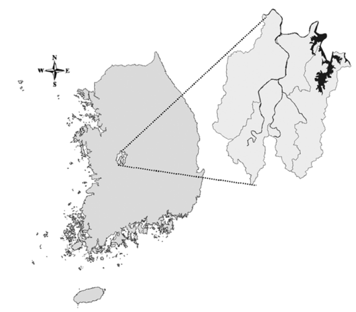
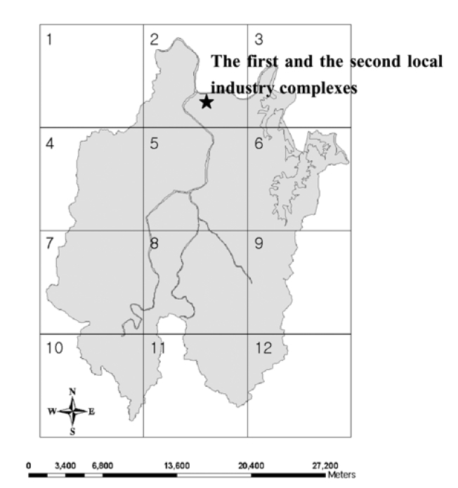
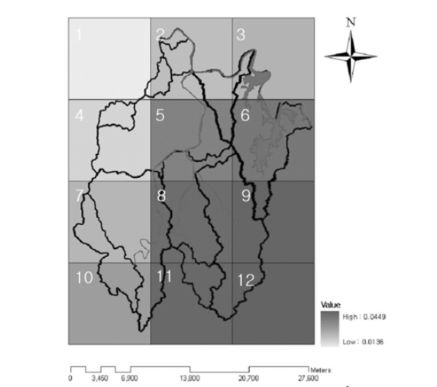
Daejeon was chosen as the study area. The city, located in the mid part of South Korea (Fig. 1), is a basin surrounded by Jikjang (eastern), Gubong (western), Bomoon (southern), and Gyejok (northern) mountains. The total area is about 540 km2 which is covered with mountain forest, urban area, rice field and farm land by 51%, 13%, 17%, and 11%, respectively (Table 1). Three streams (i.e., Gap-stream, Yudeung-stream, and Daejeon-stream) and several other small tributaries run in Daejeon. All the streams merge into Gum-river, which flows across a northern part of Deajeon. The average annual rainfall is 1,354 mm and the annual average temperature is 12.3℃. Principal wind direction is northwest at an annual average velocity of 2.42 m/sec. Two (i.e., first and second) local industrial complexes have been in operation since 1970. The industrial complexes comprise the metal, chemical, textile, and leather manufacturing plants.8) According to Korea Toxic Release Inventory (TRI),9) the two industrial complexes were the largest lead emission sources among all Korean industrial complexes. Consistently with the large emission rates, the annual average lead concentration in air was highest in 1995 and 1997 among the major cities in Korea.10)
[Table 1] Land use of Daejeon (2002)
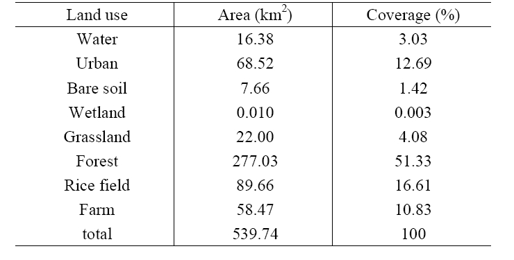
Land use of Daejeon (2002)
i.e., soils in forest, low vegetation and urban areas. The low vegetation refers to wetland, grassland, rice field and farm as listed in Table 1.
Lead could be emitted in many chemical forms which subsequently vary with environmental conditions. The major chemical form of lead in the environment includes Pb(0) and Pb(II).1) Although varying with its chemical form,1) some of the important fate and transport properties are practically similar enough to be considered the same for the modeling purposes. For instance, due to their low vapor pressure and water solubility, inorganic lead compounds exist primarily in the particulate form in air and a substantial fraction of lead in the river water is expected to be present in suspended solids (SS) bound form.1) Therefore, some of the inter-phase diffusive processes may not be significant because inorganic lead in gas or dissolved form is likely to be negligible.
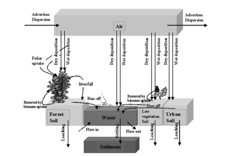
The transport processes in the model were divided into the intra-medium process and the inter-media process. The intramedium processes in the model included (1) advection and dispersion in air, (2) advection in water, (3) leaching from surface soil, and (4) sediment transport. The inter-media processes were (5) dry and wet depositions from air to soil, vegetation, and water, (6) run-off from soil to water, (7) root uptake by plants from soil, (8) foliar uptake by plants from air, (9) litter-fall of leaves to soil, and (10) settling of SS from water to sediment. The major compartments and the environmental processes linking the compartments with the chemical fluxes are depicted in Fig. 2.
A multimedia fate and transport model comprises mathematically a set of linear equations which can generally be represented as below.
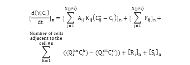
Vi : the volume of compartment i,
Ci : the concentration of the chemicals of interest in compartment i,
n : the model cell number,
Aij : the interfacial area between compartments i and j,
Kij : the i side overall mass transfer coefficient between compartments i and j,
Cij* : the pollutant concentration in compartment i which would be in equilibrium with that in compartment j,
Fij : non-diffusive cross media transport flux between compartment i and compartment j,
Qikn : volumetric flow rate of compartment i from the cell #k to cell #n,
Cik : the concentration in compartment i in the model cell # k,
k : the number of a model cell that is adjacent to the cell n,
Ri : the loss or gain reaction rate of pollutant in compartment i,
Si : the source strength in compartment i.
As the diffusive processes were negligible for the inorganic leads, the first term on the right hand side of the equation was not included in the present model.
By solving the set of the mass balance equations, the model calculates the concentration of lead in each compartment and various cross-media fluxes as necessary. The Visual Basic 6.0 (Microsoft, 1998) was used as the numerical analysis software. Input data for the model were divided into three groups, i.e., meteorological data, geographical and environmental data, and chemical data. Arc GIS 9.0 (ESRI, 1999) was used to efficiently handle the input data in the model. The watersheds were made up by using standard map of watershed provided by Water Management Information System.11) Calculation of run-off was conducted by using the Universal Soil Loss Equation.12)
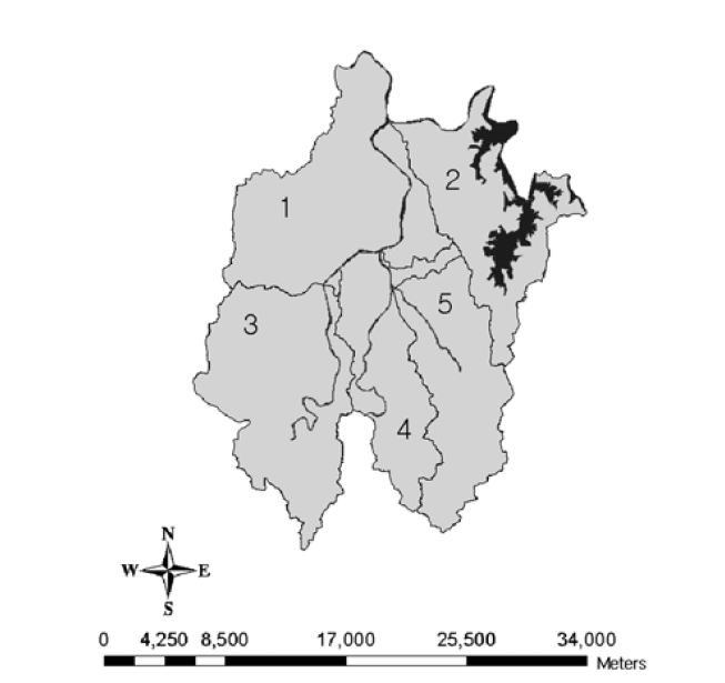
vation map and the standard map of watershed provided by WAMIS.11) As the result, a total of five watershed cells were produced (Fig. 4). Among three sub-compartments for soil (forest soil, low vegetation soil, and urban soil), forest soil was further divided into coniferous and deciduous soils to discriminate quantification of foliar uptake and litter-fall processes. The effective depth for the surface soil was assumed to be 10 cm14) while the depth of water was set at the average water depth in each watershed according to WAMIS.11)
According to Soil Groundwater Information System,15) the lead concentration in soil at a number of domestic sites which are located far from lead emission sources was negligible as compared to the contamination levels in the study area. Therefore, the background concentrations in all the compartments in this model were assumed zero.
An accurate estimation of the emission rate is critical to the certainty of the model prediction. In the present study, the reported emission rate was available only for the two industrial complexes after the year of 1999 (Korea TRI9)). In addition to the fact that the accuracy of the reported TRI values for the complexes has hardly been evaluated, the unknown lead emissions from other sources could create a great deal of uncertainty associated with the model prediction. Furthermore, since lead itself does not decompose, the lead concentration in soil at present would be strongly influenced by the past emission rate. Therefore, the emission history information was also necessary for accurate model prediction. As no such information was available, an emission scenario over the period of fifty years (from 1960 to 2010) was made up primarily on the basis of the economic growth rate, an important change in the lead regulation, the atmospheric concentration monitoring data, and TRI data9) since 1999.
2.3.1. Estimating the base emission rate in the air grid #8.
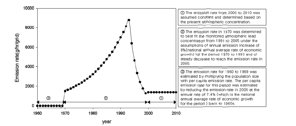
Firstly, to estimate a base emission rate (with no emission from the industrial complexes), the total simulation period was divided into four sub-periods: from 1960 to 1969, from 1970 (when the industrial complexes began the activity) to 1993 (when the use of the leaded gasoline was banned), from 1994 to 1999 and from 2000 (since when the atmospheric concentration and the TRI data became available) to 2010. The emission rate for the period of 2000 through 2010 was first determined based on the atmospheric lead concentration during 1998∼2005 in air grid #8 under the assumption that the lead emission for this period undergoes no substantial change in magnitude. The emission rate of 1378.8 g/hr/grid appeared to fit the observed level of lead in air grid #8. It was then assumed that the annual emission increased 8% over the period from 1970 to 1993 in line with the national annual average rate of economic growth for the same period (Korean Statistical Information Service, KOSIS). For the period from 1994 to 1999, it was further assumed that the emission rate steadily decreased (to account for the effect of ban of leaded gasoline16) to reach that in 2000 (i.e., 1378.8 g/hr/ grid). The emission rate of 1500 g/hr/grid has been chosen for the year 1970 among various trial values because that value along with the above assumptions resulted in the best fit of the monitored lead concentration in air grid #8 for the period from 1991 to 2005. For the period from 1960 to 1969, the emission rate was estimated by multiplying the population of Daejeon for the period (200,000) with the per capita emission rate. The arithmetic mean of per capita emission rates of Busan, Daegu and Kwangju was assumed to represent the per capita emission rate for the air grid #8. The three cities were chosen to estimate the emission rate in the urban areas of similar size without significant industrial lead emission. The arithmetic mean was first calculated for the year 2001. Subsequently, an average annual economic growth rate (7.4% from 1970 to 2000) was assumed to back calculate the emission rate for 1960s. A value of 0.530 g/hr/grid was determined for the year 1960 from the back calculation. The value might deviate from the true value because little economic growth was achieved during 1960s. The value was used without further elaboration as model calculations revealed that the lead concentration in soil for the years 2000 and later was hardly influenced by the population size or any likely values of the per capita emission rate for 1960s because the resulting emission rate for 1960s remained negligible compared to that for the later period. Fig. 5 and Table 2 show the emission estimation scheme and the background emission rate, respectively, for the air grid #8.
2.3.2. Estimating the base emission rate for other air grids
For other air grids, it was assumed that the base emission rate in each grid is proportional to the population density. The population density of each grid was approximated by the three steps, i.e., 1) estimating the sizes of land area of individual administ
[Table 2] Base emission rate for the air grid #8
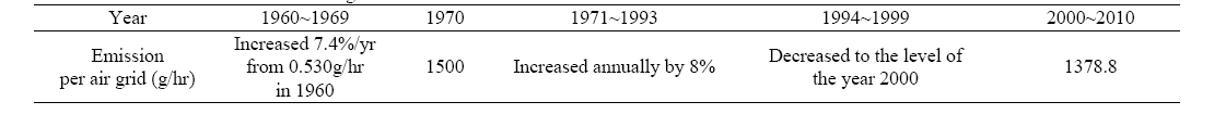
Base emission rate for the air grid #8
rative districts (Yusung-Gu, Deaduk-gu, Seo-gu, Jung-gu and Dong-gu) within each air grid, 2) allocating the population of the individual administrative districts to each grid in proportion to its size of land area that belongs to each grid, and 3) for each grid, summing up all the populations allocated from the individual administrative districts and dividing the summed population by the grid area. The first two steps described above were conducted by using GIS (ESRI, 1999). The base emission rate for each grid except #8 was then calculated by the equation below.
The base emission rate for each grid = the base emission rate of air grid #8 x population density of the grid / population density of the air grid #8
2.3.3. Estimating the additional emission rate for air grid #2
To the air grid (#2) where major emission sources are located, additional emission rate was assigned to account for the emission from the industrial complexes. The additional emission was applied from the year of 1970 when their activity began. It was assumed again that the emission rate increased annually by 8% over the period from 1970 to 1999. For the years 2000 through 2010, an emission rate of 1532 g/hr was assumed according to the average TRI emission rate for the period (Korea TRI9))The best estimate of the initial emission rate of the industrial complexes in 1970 was 152 g/hr that led to the emission rate in 2000 (i.e., 1532 g/hr). Table 3 summarizes the additional emission rate for the air grid #2 for the entire modeling period.
The model evaluation was performed in two respects, i) comparison between the measured and the model predictions for the contamination levels (relative concentration) and the atmospheric deposition fluxes and ii) sensitivity analysis.
No domestic study has been conducted to measure the wet deposition of lead. The model prediction of the wet deposition flux, therefore, was compared with those measured by Sakata et al.,22) Kim et al.,23) and Sweet et al.24) for 10 sites across Japan, Chesapeake in Delaware Bays, and Lake Superior in Michigan,
[Table 3] Additional emission rate for the air grid # 2 where the industrial complexes are located

Additional emission rate for the air grid # 2 where the industrial complexes are located
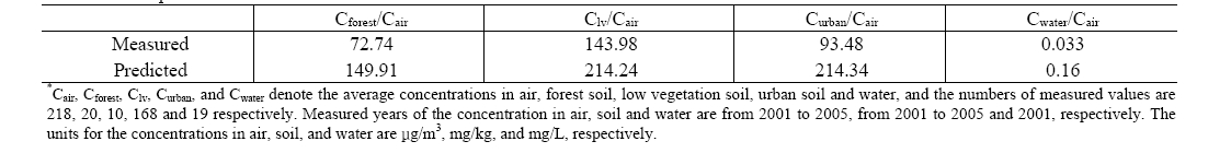
[Table 4] Comparisons of the relative concentrations

Comparisons of the relative concentrations
[Table 5] Comparison of predicted dry deposition flux with measured values (unit: μg/m2/day)
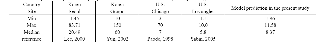
Comparison of predicted dry deposition flux with measured values (unit: μg/m2/day)
[Table 6] Comparison of predicted wet deposition flux with measured values (unit: μg/m2/yr)
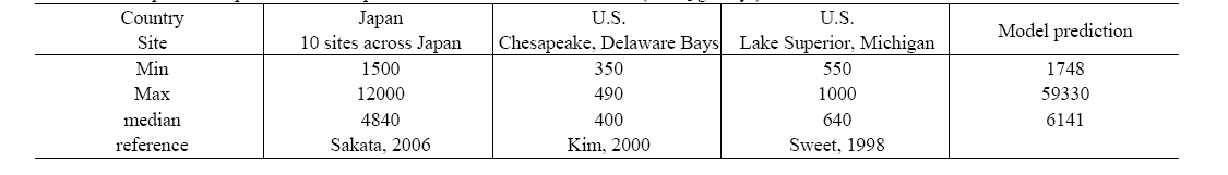
Comparison of predicted wet deposition flux with measured values (unit: μg/m2/yr)
respectively (Table 6). The model prediction of wet deposition flux was greater than those measured in the US23,24) but was comparable with the measured data in Japan.22) Again, it should be noted that the wet deposition flux also substantially varies with site.
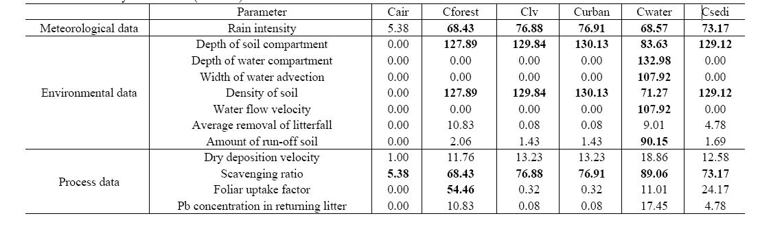
Sensitive analysis: The model sensitivity to input parameters and the model processes was assessed to identify the most critical elements of the model formulation, assessment of the uncertainties introduced by individual parameters and estimation of the overall model uncertainty.25) In this study, the sensitivity was represented by sensitivity coefficient calculated as;
Sensitivity Coefficient (%) = 'the upper value - the lowest value'/standard value × 100
where the upper value and the lowest value are annual mean values of the model outputs obtained with input data of 50% greater and of 50% lower, respectively, than the standard value.
In Table 7 summarizes the result of sensitive analysis. The result showed that precise estimation of effective volume of environmental medium was important. Also, run-off was one of the critical elements for predicting the concentration in water. Sensitivity of rain intensity and scavenging ratio were high and wet deposition flux appeared more influential than dry deposition on the concentrations in water and soil. The result also showed that the concentration in forest soil was sensitive to foliar uptake process, indicating that the knowledge on distribution and composition of trees and their ecology is substantial.
3.2. Model Prediction and Implications
[Table 7] Sensitivity Coefficients (Unit : %)

Sensitivity Coefficients (Unit : %)
strongly suggesting that atmospheric emission was the principal water pollution source in the study area. Therefore, these results imply that control of atmospheric emission is critical to protecting the quality of not only air but also other environmental media.
As shown in Fig. 7, the lead concentration in air was predicted to be highest in grid #12, and lowest in grid #1 as a result of lead transport by prevailing wind (i.e., North-West). The difference between the average concentrations in grid #1 and grid #12 was within four folds. The spatial trend of the concentration in soil matched with that in air because the contamination of surface soil occurs primarily by atmospheric deposition. The concentration in water was greatest in the watershed #1. The possible reason was that the influxes from upstream and surface runoff fluxes were greatest in the watershed #1. The range of the concentration in sediment was 1.52 mg/kg to 2.28 mg/kg. As the contamination level in sediment was in effect governed by that in soil,26) the spatial variation of the concentration in sediment followed the trend in soil.
A dynamic multimedia fate and transport model for lead was developed and assessment of the model was conducted by comparing the model predictions with the measured values for the concentrations in multi-media and atmospheric deposition flux. Given a lead concentration in air, the model could predict the concentrations in water and soil within a factor of five. The model may further be used to predict the concentrations in air, water and soil if precise emission rate is available. Sensitivity analysis indicated that the effective compartment volume should be accurately estimated. It was also noted that rain intensity, scavenging ratio, run off, and foliar uptake factor were critical elements in the precise model prediction.
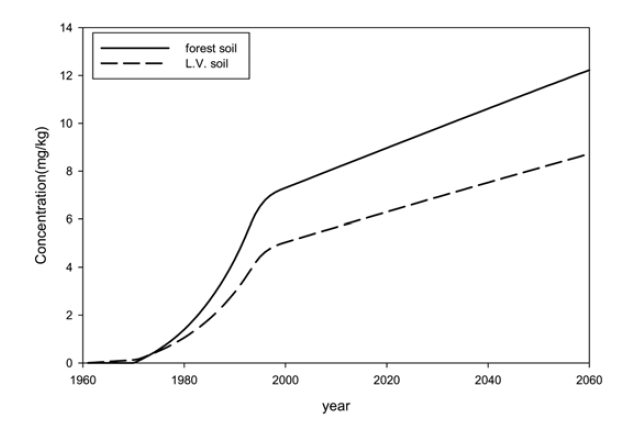
Important implications drawn from the model predictions include that i) restriction of air emission may be necessary in the future to achieve the soil quality objective as the contamination level in soil is predicted to steadily increase at the present emission level and ii) direct discharge of lead into water body was insignificant as compared to the atmospheric deposition flux, strongly indicating that the water quality (and the sediment quality) would vary principally with the air quality. In summary, due to the cross-media transfer characteristics of lead, atmospheric emission governs the quality of the whole environment. By the use of the multi-media fate and transport model developed in the present study, quantitative and integrated understanding of the cross-media characteristics is made possible and the relationships of the contamination level among the multi-media environment as a result of the cross-media characteristics could effectively be assessed.