The reduction of traffic accidents and improved road safety are important research subjects in transportation-related institutions or the vehicle industry. Driver-assistance systems (DASs) aim at bringing potentially hazardous conditions to the driver’s attention in real time [1], and they also aim at more driver comfort. Autonomous driving is also already reality in on-road vehicles [2].

At present, moving object detection and tracking is an important research subject of DASs. Usually, approaches of moving object detection and tracking first identify objects and then try to estimate the motion by tracking the objects. Dynamic scenes, the diversity of moving objects, including non-rigid body pedestrians and rigid body vehicles, as well as weather, light and other factors, make moving objects detection and tracking very difficult.

However, drivers seem to be more concerned about unusual motion regions than with moving objects in general. We suggest to detect the unusual motion regions at pixel-level rather than at moving object level. We estimate a collision risk for every single image point, independent of an object detection step.

Visual attention is one of the most important mechanisms of a human visual system. According to the visual attention mechanism, visual saliency can detect salient regions in image and video. The visual attention model, using a mathematical model to simulate the human visual system, became a “hot topic” in computer vision.

This article aims at using the visual attention mechanism to detect unusual motion for vision-based driver assistance. The remainder of this paper is organized as follows. The unusual motion detection framework is presented in Section 2. Section 3 describes salient region detection based on visual attention. Section 4 introduces unusual motion detection within the detected salient regions. Section 5 presents the experimental results. Finally, Section 6 concludes the paper and opens perspectives for future work.

In DASs, unusual motion detection is one of the important means of preventing accidents. Motion detection techniques often rely on detecting a moving object before computing motion [3]. The performance of such methods greatly depends on the performance of moving object detection.

It is a common human experience of getting out of the way of a quickly moving object before actually identifying what it is [1]. In conclusion, a human can perceive motion earlier than form and meaning.

In this paper, we propose an unusual-motion-detection model for vision-based driver assistance. The proposed model is able to detect the collision risk for the considered image points, that is independent of an object detection step.

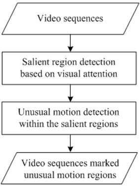
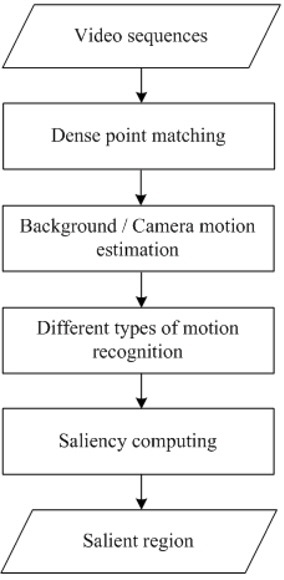
Figure 1 illustrates our proposed unusual-motion-detection framework. This framework contains two stages, salient region detection based on visual attention, and unusual motion detection within the detected salient regions.

Since directly computing pixel-level unusualness is computationally expensive, we first introduce a salient-region-detection method, so as to define the unusual-motion-detection areas. In the stage of salient region detection, an improved temporal attention model is proposed to detect the salient regions.

In the second stage, three different factors, the speed, the motion direction, and the distance are considered to detect the unusual motion for every pixel within the detected salient regions.

In video sequences, motion plays an important role and human perceptual reactions will mainly focus on motion contrast regardless of visual texture in the scene.

Visual saliency measures low-level stimuli to the human vision system that grab a viewer’s attention in the early stage of visual processing [4]. While many models have been proposed in the image domain, much less work has been done on video saliency [5].

Zhai and Shah [6] proposed a temporal attention model to use the interest point correspondences and the geometric transformations between images. The projection errors of the interest points, defined by the estimated homographies, are incorporated in the motion contrast computation.

Tapu and Zaharia [7] extended the temporal attention model. Different types of motion presented in the current scene are determined using a set of homographic transforms, estimated by recursively applying the Random Sample Consensus (RANSAC) algorithm, see [8, 9], on the interest correspondences.

In the previously developed methods, detecting the feature points is the first and most important step. Obviously, the performance of the temporal attention model is greatly influenced by the results of point correspondences [10]). The Scale Invariant Feature Transform (SIFT) is used to find the interest points and compute the correspondences between the points in video frames; see also [9] for a description of SIFT.

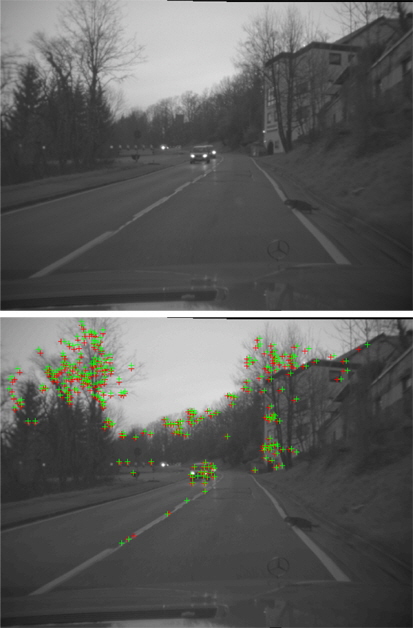
However, it is well known that the interest point distribution generally represents a rich texture information area. If there is less texture in the potential object regions, then there are no feature points to be detected in these regions and thus the potential object regions cannot be detected. An example of interest points, detected by SIFT, is shown in Figure 2. In this case, the region where the cat (running right to left) is located is the potential object region. As shown in Figure 2, most of the detected interest points are located in the background.

In this stage, we extend the temporal attention model, proposed by Zhai and Shah [6], to obtain dense point correspondences based on dense optical flow fields. The optical flow technique is the most widely used motion detection approach [9, 11]. Optical flow at edge pixels is noisy if multiple motion layers exist in the scene.

Furthermore, in texture-less regions, dense optical flow may return error values [6]. To overcome this problem, we use a RANSAC algorithm on point correspondences to eliminate outliers.

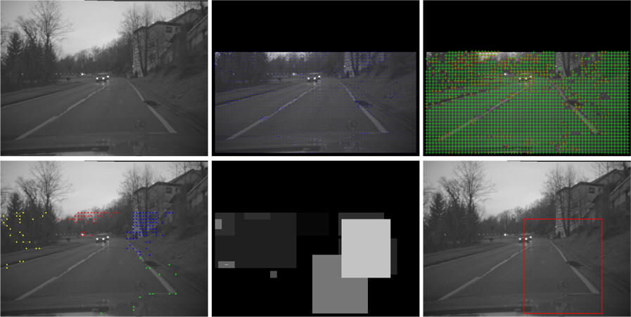
As shown in Figure 3, this stage consists of the following steps:

Step 1: Dense point matching - First, the dense optical flow method TV-L¹ [12] is used on two consecutive frames to calculate the dense point correspondences at 10-pixel intervals. Since the moving objects always appear on the lower part of the input frames, the dense optical flow method is applied only to the bottom two thirds of the input frames. This reduces the computation time. Furthermore, to avoid the effect of noise, we exclude a 10-pixel-wide border around every frame.

Step 2: Background / Camera motion estimation - Obviously, most of the points detected at Step 1 are located in the background. The subset of m background points can be determined with the epipolar geometry constraints.

We use the multi-view epipolar constraint which requires the background points to lie on the corresponding epipolar lines in subsequent images.

If the points are far away from the corresponding epipolar lines, then we can determine them as being foreground points.

For the spatial point correspondences detected at at Step 1, we apply a RANSAC algorithm respectively to determine the fundamental matrix F.

Step 3: Different types of motion recognition - In practice, multiple motions are present that result from the moving objects, but also from background objects or camera movement.

In this case we determine a new subset of points formed by all the outliers and all the points not considered in previous step.

For the current subset, we apply a RANSAC algorithm recursively to determine multiple homographies until all the points belong to a motion class. The estimated homographies model different planar transformations in the scene.

Every estimated homography H_m has a set of points as its inliers, and n_m is the number of inliers for H_m.

For every homography H_m, its inliers in L_m can be considered as being located in the same plane. However, the points may belong to a distributed region.

To avoid the problem, we use the K-means clustering algorithm to divide L_m into K subsets, , for i = {1,...,K}. The spanning region of L_m,i is denoted by R_m,i, which corresponds to a moving region.

Step 4: Saliency computing - For all the moving regions determined at Step 3, we compute now their projection errors as saliency value.

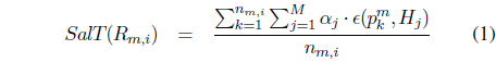
The temporal saliency value of the moving region R_m,i is defined by

where M is the total number of homographies in the scene, is the projection of computed after applying H_j, is the correspondence of found by TV-L¹ , and α_j,i is the spanning area of the subset L_j,i.

An example of salient region detection based on visual attention is demonstrated in Figure 4, where apparently the attention region in the sequences corresponds to the running cat.

In the first stage, detecting the salient regions to define the unusual motion search area can reduce the computation time. In this stage, we detect the unusual motion within the detected salient regions.

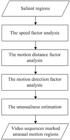
We analyze the unusualness for every pixel from the following three factors: the speed, the motion direction, and the distance. As shown in Figure 5, this stage consists of the following steps:

Step 1: The speed factor analysis - The optical flow technique can accurately detect motion in the direction of intensity gradient and is the most widely used motion detection approach [11]. The TV-L¹ method is one of the best optical flow methods proposed in recent years [13]. The optical flow features in each detected salient region are obtained using the TV-L¹ method [12].

Intuitively, the speed is a determining factor in judging the unusualness of a pixel. Let (v_x, v_y) be the motion vector at a pixel location (x, y). Therefore, the unusualness value U_s(x, y) at pixel location (x, y) can be defined as follows:

where D_min and D_max are the maximum and minimum value of magnitude, respectively.

Step 2: The motion distance factor analysis - Since only motion within some distance range is interesting for the driver, we enhance effects of motions within an assumed distance range, and decrease the impact of motions outside of this distance range. We use the general weighted operator of [14] to calculate the weight value of the motion distance factor w_d(α_d, d) as follows:

where d is the spatial distance between the pixel location (x, y) and (w/2 ,h), which is normalized to [0, 1]. Here, e_d is the threshold of the motion distance, n is − ln 2/(ln(1 − α_d) − ln 2) with α_d in the range of [0, 1], and α_d controls the strength of motion distance weighting. Larger values of α_d increase the effect of motion distance weighting so that the closer motion would contribute more to the unusualness of the current pixel.

Step 3: The motion direction factor analysis - The motion direction is another factor in considering the unusualness for every pixel. Figure 6 illustrates the motion direction for every pixel within the salient regions.

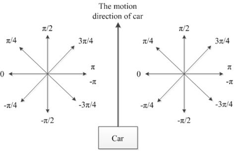
As shown in Figure 6, the host vehicle is in the bottom middle of a frame. Intuitively, for the left-half region, we should just consider those pixels with the motion directions in [−π, −π/2] or [π/2, π]. Similarly, for the right-half region, we should just cope with the pixels with motion directions in [−π/2, π/2].

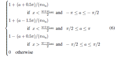
In practice, to deal with the width of the host vehicle car, we will adjust the right and left region. The weight value w_a(α_a, a) of the motion direction factor is defined as follows:

where a is the motion direction at the pixel location (x, y), w_car is the width of the host vehicle, and α_a controls the strength of motion direction weighting. Larger values of α_a increase the effect of motion direction weighting.

Step 4: The unusualness estimation - Based on all the factors determined in the steps before, we compute the unusualness value U(x, y) at pixel location (x, y) as follows:

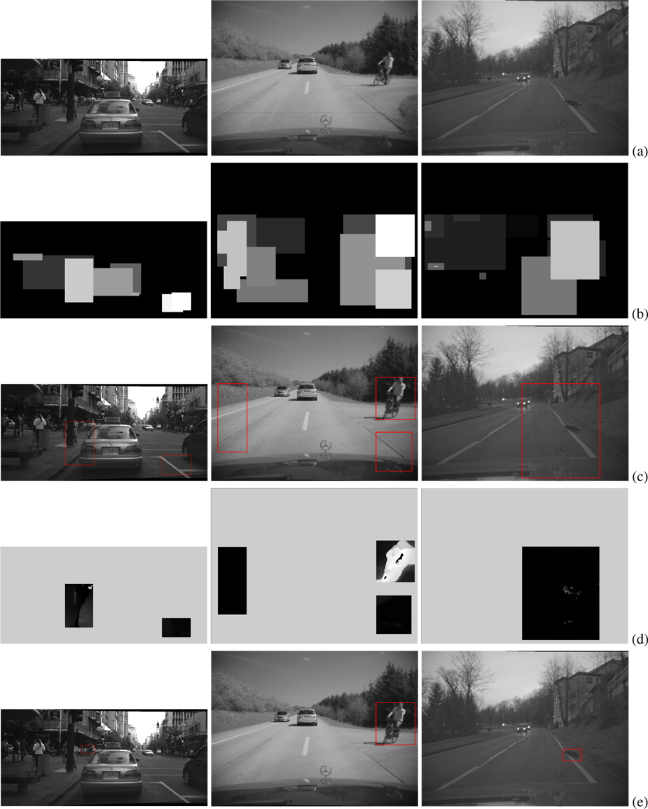
To evaluate the performance of the proposed unusual-motiondetection model, we conducted experiments on different kinds of video. A few detailed results are shown in Figure 7. The following information is presented: the representative frames of the testing videos (Figure 7a), the temporal saliency maps of the representative frames (Figure 7b), the detected salient regions (Figure 7c), the unusualness maps of the detected salient regions (Figure 7d), and the regions that correspond to potentially unusual motions (Figure 7e).

In this paper, we have developed a model for detecting unusual motion of nearby moving regions. The model can estimate the unusualness for an output of warning messages to the driver to avoid vehicle collisions. To develop this model, two stages, salient region detection and unusual motion detection, were implemented.

Based on spatiotemporal analysis, an improved temporal attention model was presented to detect salient regions. Three factors, the speed, the motion direction, and the distance, were considered to detect the unusual motion within the detected salient regions. Experimental results show that the proposed real-time unusual-motion-detection model can effectively and efficiently detect unusually moving regions.

In our future work, we plan to extend the proposed method by taking into account not merely successive frames, but also some accumulated content (e.g. about the traffic context) of a video in order to increase the robustness of the algorithm and to incorporate an object tracking method.