Despite broad globalization pressures, import tariffs in agricultural and food industries remain particularly high compared with the industrial sector. The Organization for Economic and Co-operation Development (OECD) estimated that the average tariff for agricultural and agri-food products in OECD countries was 36% (OECD, 2003).1 In comparison, tariffs on industrial products fell from an average of 40% after the Second World War to nearly 4% (OECD, 2002). Unfortunately, the lessons from this spectacular exercise in trade liberalization have not inspired the members of the World Trade Organization (WTO) to pursue a path of rapid trade liberalization for agricultural products. In spite of the tariffication process undertaken in the Uruguay Round (UR), Non-Tariff Barriers (NTBs) remain important impediments to agri-food trade (UNCTAD, 2005). Furthermore, several countries support agriculture with production subsidies and supply controls. On the positive side, the potential trade-distorting effect of domestic subsidies was recognized in the UR and, as a result, ceilings are imposed on subsidies that are tied to current production.

Many agricultural products can be exported as primary or processed commodities (e.g. wheat versus flour, soybeans versus oil, livestock versus meat, and so on). This is important for policy analysis purposes because primary and processed products are often taxed or subsidized at very different rates and because a policy directed at one type of product will have an incidence on the other type through vertical production linkages between primary and processed products. Tariff escalation is a common phenomenon. It is most evident in the schedules of Eastern Europe and the Middle East, followed by North America, South Asia, and the EU for products such as meats, sweeteners and vegetable oils (Gibson et al., 2001, p. 22) . Higher taxes on processed products tend to increase demand for domestic and imported primary products. So a fall in processed products imports is likely to be accompanied by an increase in primary products imports, unless a tax on primary products or NTBs prevent such adjustments. Therefore, one could mistakenly conclude when looking at aggregate data that a tariff does not have much of an impact when, in reality, substantial changes in the flows of traded processed and primary products offset one another. This shows the importance of disaggregating primary and processed products when analyzing agricultural trade liberalization.2

Another reason to use disaggregated products by stage of production is that trade in processed products has been growing much faster than trade in primary products. The share of processed products in the world’s agricultural exports has increased from 42% to 48% between 1990 and 2002. This applies to most exporting countries, except some of the poorest ones and Brazil and Chile, which have a strong comparative advantage in the production of primary products. The faster (slower) growth in trade of processed (primary) products occurred in spite of tariff escalation, but under notoriously significant NTBs on primary products.

In the Doha Round, Developing Countries (DCs) have shown resolve in their quest to obtain significant concessions on agricultural issues from developed countries. Many DCs may wish for better access to developed countries’ markets for agricultural and food products to exploit their comparative advantage. The EU, the US, Japan (and China) are among the top five destinations for agricultural exports of many DCs and developed countries.3 For these DCs, developed countries’ protectionism in agriculture hinders their economic growth.4 In the context of the multilateral trade negotiations, it is important to understand how welfare gains evolve along various trade liberalization paths for primary and processed products and to assess the welfare impacts of other trade impediments and the degree of product differentiation in processed products. Few papers have analyzed trade policy in vertically-related markets (notable exceptions include McCorriston, 2002; and McCorriston & Sheldon, 1996) and in most cases they have ignored product differentiation in the downstream market while assuming that trade in the upstream market is hampered only by standard trade taxes.

The objective of this paper is to analyze the welfare implications of different liberalization paths in agri-food sectors accounting for potential NTBs in agriculture as well as vertical relationships between farm output and downstream industries. The theory of the second-best tells us that some liberalization from a distorted equilibrium need not increase welfare. The implication is that small reductions in some tariffs and/or in domestic support in highly distorted agricultural markets may decrease welfare. For example, let us take the case of an importing country that reduces its production subsidy on primary products. This should bring about a reduction in the domestic supply of primary products. If there are NTBs and imports of primary products do not increase, the production of local processed product will fall and this could bring about a substantial decrease in consumer surplus and overall welfare if the domestic processed good is highly differentiated from imported ones and has an inelastic demand. In this context, fairly large tariff reductions would be needed to counter NTBs and trigger enough substitution away from domestic primary and processed goods to increase welfare.

As argued by Copeland (1990), it is not always possible for negotiations to encompass or be as aggressive on all policy instruments. In the UR, advances were made on market access, domestic support and export subsidies. There is now a consensus on the elimination of the latter, but the first two are still the object of much dissension. Some authors have investigated the issue as to which between tariff reductions and domestic support reductions ought to be chosen if negotiationswere to focus on only one of these policy instruments. Hoekman et al. (2004) contrast the impacts of reducing import tariffs versus domestic support on DCs’ exports and found that a 50% cut in tariffs has a much larger impact on exports than a 50% reduction in domestic support. The relative potency of tariff reductions is not surprising in their context because tariffs can be likened to simultaneous imposition of a production subsidy and a consumption tax (Bhagwati et al., 1998, p. 262).

Our theoretical framework builds on the recent literature on gravity models5 by modeling trade of differentiated processed commodities while considering transaction costs and export supply rigidities at the farm level that may arise due to the presence of NTBs (UNCTAD, 2005). We rely on numerical simulations to illustrate the impacts of tariff and/or domestic support reductions on the volume of trade and prices, linking the overall welfare implications of trade liberalization to rigidities in the agricultural export supply functions and product differentiation in food products.

We show that the introduction of NTBs, vertical linkages and product differentiation at the processing level can reverse the welfare ranking of tariff and domestic reductions.We also show that depending on where countries are on the liberalization path, tariff and domestic support reductions may mitigate or boost each other’s welfare effects. Thus, we bring new insights about the impacts of trade liberalization on agri-food trade flows and welfare. Because many models use highly aggregated data and transform all policies into tariff-equivalents, they cannot analyze with precision the welfare implications of trade liberalization for vertically-related products in the presence of different policy instruments.

The remainder of the paper is structured as follows. The next section lays down the theoretical foundations of our modeling framework. Section 3 describes a three-country model derived from our modeling framework that easily lends itself to simulations. It is easier to extract intuition froma simple low-dimensional model, but the model must impose theoretically consistent vertical linkages between primary and processed products and it must also have a rich enough policy space to isolate the respective effects of tariff and domestic support reductions under different assumptions regarding NTBs and product differentiation. In our framework, tariff reductions in developed countries are not always more effective than domestic support reductions in enhancing a DC’s welfare. By having two developed countries and one DC, we can also capture stylized facts about North–North and North–South trade and derive insights about the position of DCs regarding agricultural trade liberalization. Results from our simulated trade liberalization scenarios are presented in Section 4. The final section summarizes key results and their implications.

1The peaks of agricultural tariffs are also a cause for concern. Bchir et al. (2005, p. 21) show that the shares of products with an average bound tariff in excess of 100% are 5.8% and 12.1% for developed and developing countries, respectively, but there is much variation between countries. The same statistics for China, Mercado Común del Sur (MERCOSUR) and India are respectively 0%, 0% and 43.7% while for the United States (US) and the European Union (EU), we have 0.4% and 5.1%. Anderson (2009) provides a detailed account of the evolution of agricultural distortions in different parts of the world.   2As pointed out by an anonymous reviewer, Computable General Equilibrium (CGE) models offer rich linkages between agricultural and non-agricultural sectors, but they often fail to account for variety (except through an Armington aggregator for intra-industry trade) or even for NTBs unless they are embedded in tariff equivalents. In the latter case, the effects of NTBs cannot be analyzed separately. Most gravity models also use a high level of product aggregation. As a result, little is known about how trade liberalization operates when specifically accounting for vertical linkages between primary and processed products.   3As pointed out by a referee, the top five destinations for EU agricultural exports, Russia, Saudia Arabia, China, Turkey and Algeria, stand out vis-à-vis the top five destinations of other countries.   4Other DCs may be tying reductions in their own non-agricultural tariffs to concessions on market access and domestic support for agricultural products to limit their concessions on non-agricultural tariffs, thus hoping for a timid Doha outcome.   5Leamer and Levinsohn (1995) argue that gravity-based models have produced some of the clearest and most robust results in the economics science. See Eaton and Kortum (2002), Evenett and Keller (2002), Debaere (2005) and Helpman et al. (2008) for insightful applications of the gravity model. Anderson and van Wincoop (2004) provide an excellent survey of the literature.

The description of our model begins with the primitives about consumer preferences and processing and primary production technologies that condition consumer and firm behaviour. We then specify market-clearing conditions from which we derive economy-wide functions before defining and characterizing the equilibrium. In the process,we discuss assumptions made to ensure that regularity conditions hold for comparative static purposes. We then discuss the additional assumptions behind the empirical version of the model from which we perform numerical simulations.

We assume that there are Z (z = 1, . . . , i, j, . . . ,Z) countries in which consumers  have identical preferences over a certain processed good. There are N_z varieties of the good produced in country z. Consumers’ preferences in each country are summarized by a CES-type utility function over varieties.6 Let q_iz(ω) be country i’s consumption of the good produced in country z with ω indexing varieties. Let the parameter η > 1 measure the elasticity of substitution between varieties. The utility function being maximized by consumers is:

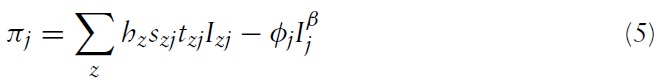
Under the assumption of monopolistic competition in the production of the processed good and constant average variable costs, profit maximization implies:

where p_z is the price received by firms in country z, and c_z is the marginal cost of production in country z that depends on the technology described below. Using equation (2), country i’s demand function for the variety of a processed good supplied by country j is:

where Y_i is the aggregate income in country i, α is the share of income spent on a processed good and τ_ij ≥ 1 represents trade costs (tariffs, transportation, etc) associated with shipping to location i from country j. For the time being, it is assumed that income is exogenous. Imports in country i are equal to the aggregate consumption of each variety times the number of varieties:

It is useful at this stage to introduce a little more structure on the technology to simplify the simulation exercise carried out in the next section. More specifically, it is assumed that the production function for a processed commodity has a Cobb-Douglas form:

where TFP_j is the total factor productivity specific to each country, and L_j and I_j respectively denote labour and the quantity of primary good used in the production of a processed good in country j. Factor prices in country j are respectively denoted by w_j and h_j. The supply of labour is perfectly elastic from the perspective of agri-food firms and thus they perceive w_j as a constant. Under these assumptions, marginal cost in country j is: c_j =

where

Although primary products are homogeneous, they are not likely to be freely substituted between foreign markets from the exporting country’s perspective. Many of the reasons motivating the imperfect substitutability of primary agricultural products across destinations revolve around NTBs. For example, agricultural products often need to meet sanitary or packaging criteria that can differ across importing countries. It could also be that importers have particular demands related to delivery that discourage destination switching.7

Assume that the production function of the agricultural good is homothetic and let I_j denote country j’s production of the primary good while φ_j denotes a cost parameter. The cost function of a representative agricultural producer in country j can be depicted as:

with β > 1. Following Geraci and Prewo (1982) and Baier and Bergstrand (2001), the aggregate output of the primary good is:

where γ is the constant elasticity of transformation (CET) introduced by Powell and Gruen (1968) to analyze agricultural supply. If γ is zero, primary products cannot be substituted across destinations while a value of infinity implies that products can be freely substituted. A distinguishing feature of our framework is that we interpret the CET function as a cost function and not simply as an aggregator function.8

Profits of agricultural producers are defined as:

where s_zj ≥ 1 is the production subsidy equivalent in the primary sector offered by country z, t_zj ≤ 1 measures the bilateral trade costs for the primary product and h_z is the price of the primary product received by producers in country z.9 Note that the production subsidy offered in country j is also indexed according to the destination of the primary product. In theory, domestic support should not be conditional on the ultimate destination of the product, but introducing this notation serves two purposes. First, the subsidy equivalent is measured as a percentage of the domestic price in destination zand domestic prices vary across destinations. Second, the variable s_zj can be adjusted to account for both export and production subsidies.

Sale revenues in market z are derived from the price received in market z plus the support offered by country j minus the transaction cost of shipping the product from j to z. Note that the notion of homogeneity among primary goods is supported by the condition that the price received in market z is independent from the origin of the product. However, goods are not homogenous in a ‘pure’ sense because they cannot be freely substituted across destinations from the producing country’s perspective. Hence, the rigidity in trade originates from the technological side and, as a result, there is no arbitrage condition between prices of the primary good in any given market (i.e. h_z ≠ h_z’∀z ≠ z’).

Consider the profit maximization problem of a representative primary producer in country j. Profit maximization yields the following set of first-order conditions:

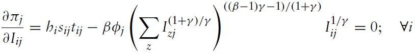
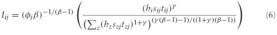
Solving the full system of first-order conditions yields the following bilateral export supply equation from country j to country i:

Note that we must have γ > 1/(β − 1) for the second-order conditions to hold. This inequality states that destinations can be substituted relatively freely (low NTBs associated with a high γ ) only if decreasing returns to scale are not too large (as measured by the parameter β). This ensures that the export supply function from country j to destination i is increasing in the price (h_i) paid in market i(∂I_ij/∂h_i > 0 for j ≠ i) and decreasing in prices observed in other destinations.

Vertical linkages at this stage are introduced through a series of market clearing conditions. Given the assumptions about technology, the conversion factor between the primary and the processed goods in country j is

The market clearing conditions restrict country j’s total purchase of primary goods to be equal to its (proportionally adjusted) shipments of the final good to all destinations:

In all, there are Z equilibrium conditions that solve for primary good prices in Z countries.

6Consumers’ preferences in each country could also be summarized by Cobb-Douglas preferences over goods. This would be consistent with two-stage budgeting and a partial equilibrium framework.   7Rauch and Feenstra (1999) discussed these costs in a context of networks in international trade.   8The microeconomic foundations of this cost function become clearwhen considering the following two-stage production process: In the first stage, each firm produces an aggregate output that is subsequently tailored to each particular market in a second stage. Customizing the aggregate output leads to less (more) individual destination-specific output assuming that γ < (>)0.   9The link with the usual rate of subsidy κij ≥ 0 can be recovered through sij ≡ 1 + κij ≥ 1. Similarly, we can relate the usual ad valorem tariff Tij to the trade cost measure through tij ≡ 1/(1 + Tij) ≤ 1. An increase in tij can be interpreted as a decrease in the ad valorem tariff.

Because of the presence of vertically constrained primary and processed sectors, supply-side rigidities in the export of primary products, product differentiation in the markets for processed products and many countries, the effects of tariff and domestic support reductions are too complex to be analyzed analytically. As a result, we follow Abrego et al. (2006) in relying on numerical simulations to provide insights regarding the welfare implications of various liberalization scenarios in a second-best environment. Sensitivity analyses allowus to ascertain the relative and absolute importance of parameters governing supply-side rigidities and product differentiation on welfare outcomes. The welfare analysis is carried out in a partial equilibrium framework that can be reconciled with quasi-linear preferences with a manufactured good being the numéraire.

There is little arguing that the US and the EU are the two most important economic powers and that they both heavily subsidize agriculture. As such, one or the other is the main trade partner for a very large number of smaller countries. Consequently, a three-country trade model is the simplest structure allowing us to investigate agricultural trade liberalization scenarios from the perspective of a small developing open economy. It should be noted that the label ‘small’ only refers to the size of the economy and not to the usual assumption about the ability of a country to influence its terms of trade.

The downstream food processing firms combine the primary agricultural goods with labour to produce the processed good/food. It is assumed that the price of labour is exogenous to the agri-food sector10 and that income in the developing economy, also referred to as the third country or DC, is five times lower than the income in the large countries. The third country is heavily dependent on export markets and does not support its agricultural sector with coupled subsidies. Hence, s₁₃ = s₂₃ = s₃₃ = 1 is observed in country 3 while s₁₁ = s₂₁ = s₃₁ = s₁₂ = s₂₂ = s₃₂ = 1.5 in the two large economies. The import tariffs in the upstream agricultural sector of countries 1 and 2 are set such that they yield a tariff-equivalent measure of 50%; hence t₁₂ = t₁₃ = t₂₁ = t₂₃ = 1/1.5 = 0.67. The trade costs in the downstream agri-food sector of countries 1 and 2 are set to τ₁₂ = τ₁₃ = τ₂₁ = τ₂₃ = 2 which imply 100% ad valorem tariffs. Country 3, the DC, pursues a free trade policy.

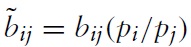
The above baseline values were purposely chosen to portray tariff escalation as higher duties are applied on processed products and lower duties are applied on primary goods. Tariff escalation measures are often based on the effective rate of protection, but the validity of such measures is questionable when the small country assumption does not hold (Golub & Finger, 1979). The Effective Rate of Protection (ERP) of product j is computed as:

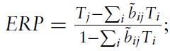
where T_j is the tariff applied on product j,

and the b_ij’s are input–output coefficients. When terms of trade are endogenous, as in our framework, a better measure of tariff escalation is the tariff wedge between input i and output j: TW = T_j − T_i. When the processed product is more protected than the input TW > 0 and ERP > T_j > T_i > 0.

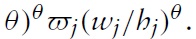
There are three market clearing conditions in our three-country model:

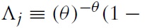
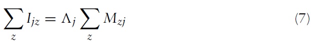
whereas before, ˄_k is the conversion factor between the primary and the processed goods. It is assumed that tariff revenues are transferred to consumers in a lumpsum fashion and that export and domestic subsidies are financed through lumpsum taxation. Hence,welfare is measured as the sum of consumers’ surplus, firms’ profits and net government revenues.The latter termincludes tariff revenues minus subsidy payments:

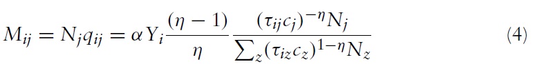
The market clearing conditions in equation (8) and the import demand and export supply functions defined in equations (4) and (6) provide the necessary structure to solve for the three endogenous prices {h₁, h₂, h₃}.

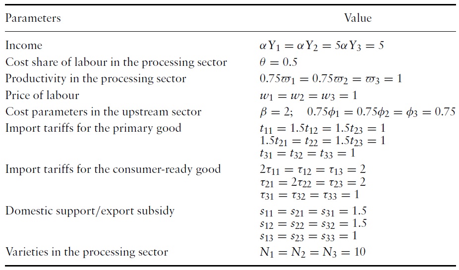
Table 1 lists the actual values of each parameter used in the baseline solution. The structural parameters pertaining to countries 1 and 2 are assumed to be identical. However, differences in cost structure are introduced between the two large countries and the DC (country 3). Specifically, it is assumed that country 3 has a cost advantage in the downstream and upstream agri-food sectors. Several DCs, like Brazil and Argentina, are major competitors on world markets for a wide array of products ranging from soybeans and soybean oil to cattle and beef and chicken and poultry meat. The cost advantage given to the DC could be construed as ‘stacking the cards’ to produce large gains from trade liberalization but, as will soon be shown, this presumption make our subsequent results all the more intriguing. In the simulated liberalization scenarios, we allow parameters γ and η to vary. The former measures the degree of substitution across export markets for primary agricultural goods (i.e. low substitution implies significant NTBs in the upstream sector) while the latter measures substitution between country-specific varieties of processed goods.11

Three scenarios are simulated. In the first, linear cuts are applied to domestic support holding tariffs constant. In the second, linear tariff cuts are applied while holding domestic support constant. Cuts are assumed to be applied in ten equal incremental steps until free trade is achieved, starting from an initial domestic support value of 50%. Similarly, tariffs on processed and primary goods are respectively cut from their initial values of 100% and 50%. Note that tariff escalation remains along the liberalization paths, but the extent of tariff escalation (measured by TW) is reduced as tariffs converge to zero.12 Finally, an ambitious liberalization scenario is simulated in which domestic support and tariffs are decreased simultaneously.

10The exogeneity of wages is a realistic assumption for developed countries, but it is less so for developing countries that have fairly important agricultural and food processing sectors.   11Anderson and van Wincoop (2004) consider elasticities of substitution in excess of 10 as unrealistic. Thus, our two values {2,8} were selected to provide variation within a realistic range. The parameter capturing the restrictiveness of NTBs for primary products takes on the same values. Preliminary econometric results in a companion paper pertaining to the cattle/beef industry suggest that null hypothesis γ = 2 cannot be rejected. It was decided to use a value of 8 to assess the robustness of our results.   12François and Martin (2006) examine various market access reforms and their impact on tariff escalation. For example, they find that the Swiss formula is more effective than linear tariff cuts in reducing tariff escalation.

This section presents numerical simulations based on a three-country version of the framework introduced in the previous section. Our objective is to investigate whether it is preferable to have large policy-active countries lower tariffs or domestic subsidies on agricultural goods from the perspective of the developing economy. It is generally recognized that tariffs are more distorting than domestic support policies because they distort both production and consumption decisions.13 As such, one could be tempted to conjecture that negotiators should pursue more aggressively tariff reductions than domestic support reductions. However, the argument favouring tariff reductions is less evident when one considers that supply-side rigidities and NTBs are pervasive in the agricultural sector and that vertical linkages between primary and processed goods can drastically impact on the effects of tariff reductions. In particular, partial tariff liberalization scenarios and less than comprehensive disciplines on domestic support may cause situations in which disciplining domestic support yields greater benefits than tariff reductions. The parameter γ plays a key role on the direction and magnitude of the effects induced by changes in policies targeting primary goods because it creates a ‘partner bias’. A low value of γ implies that producers of the primary good and processing firms in any given country are more dependent on each other because primary goods are not as easily transferable between markets. Conversely, a high value of γ implies that primary good suppliers can supply all countries without making significant adjustments to their product.

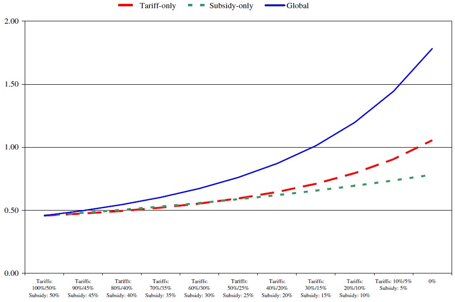
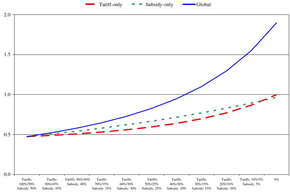
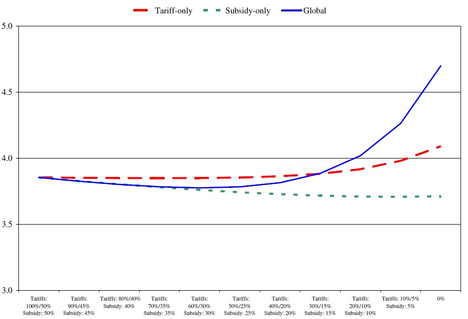
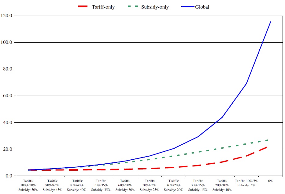
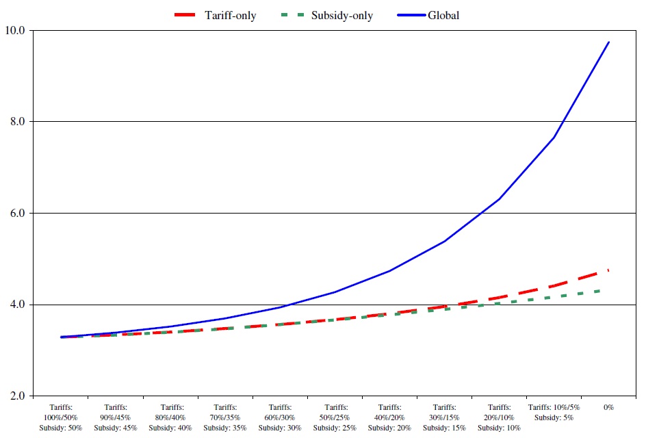
Figure 1 illustrates the evolution of the DC’s welfare when tariffs and/or domestic support is reduced and γ and η are set to 2. Reductions in domestic support have adverse effects on the welfare of the DC if tariffs are held fixed. Early on in the tariff-only liberalization scenario, tariff cuts also decrease welfare, but tariff cuts have the desired positive effects once the liberalization process has reached the half-way mark. Gains from the more ambitious liberalization scenario are observed even later, that iswhen the tariff on processed (primary) goods is reduced to 30% (15%) and the subsidy is reduced to 15%. It is also interesting to note that tariff-only liberalizationwhen tariffs and domestic subsidies are high is better than global liberalization.

The results in Figure 1 reflect the declining significance of the benefits accruing to processing firms in the DC as production subsidies offered by large countries decline. The relatively low value of γ implies that agricultural producers in the small country are confronted with significant NTBs and cannot easily increase their export sales when domestic support is lowered in the large countries. Consequently, the price of the primary good in the DC increases rather modestly as liberalization progresses, as illustrated in Figure 2. Agricultural producers benefit from higher prices, but downstream firms in the DC must cope with higher marginal costs. The price of processed goods in the DC reacts to this cost-push effect, and more so under the tariff-only scenario, as illustrated in Figure 3.

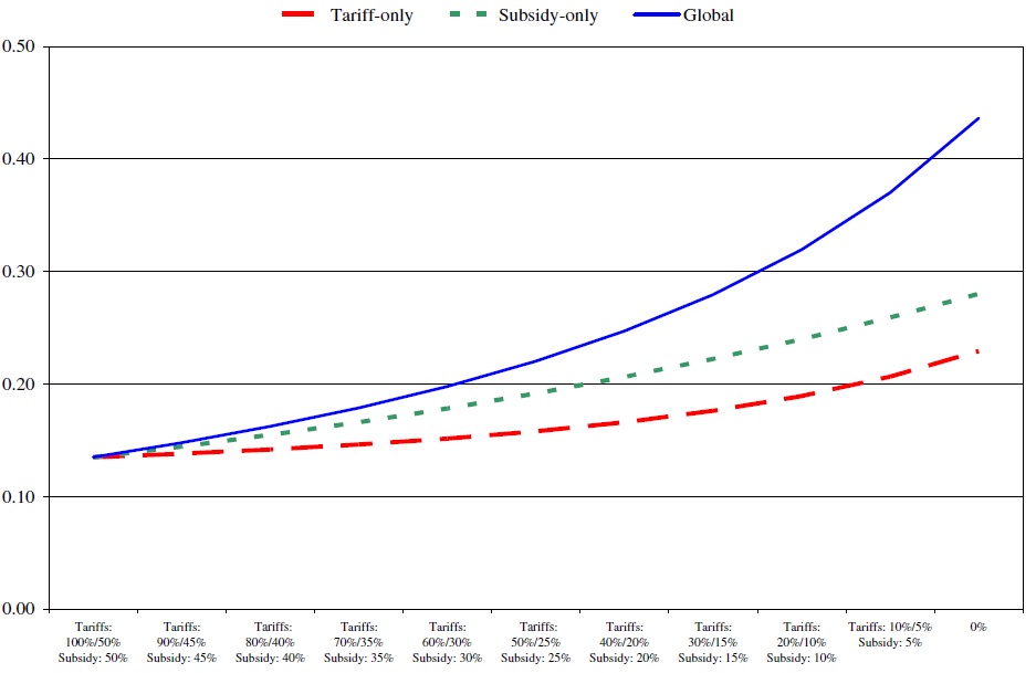
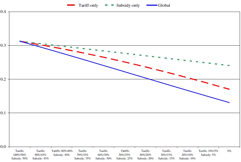
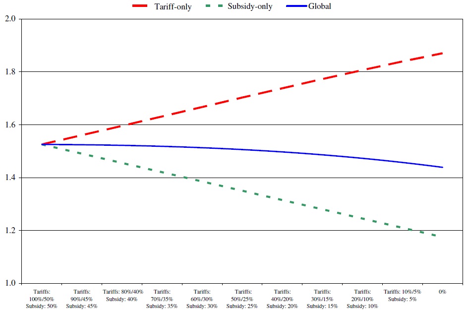
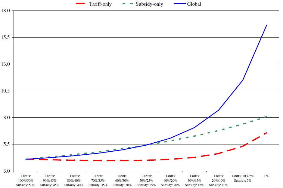
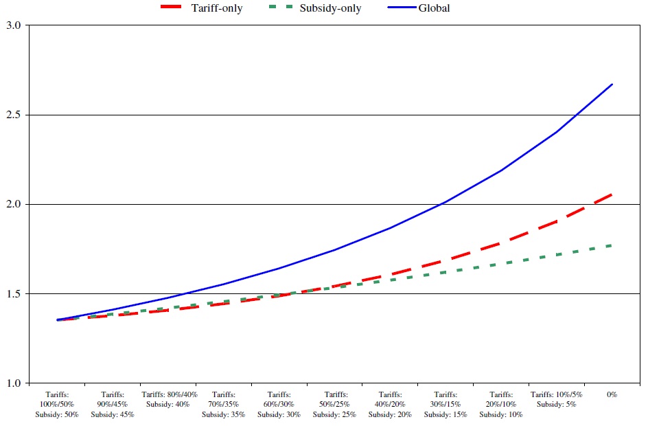
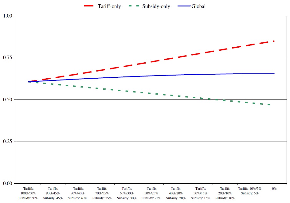
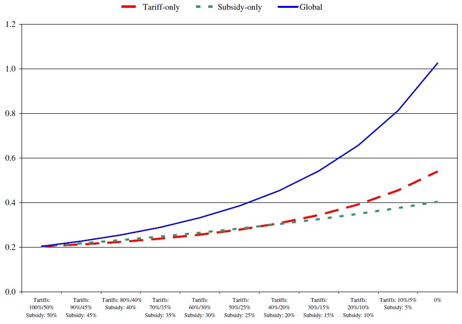
Figures 4 and 5 show the evolution of country 3’s exports of primary and processed goods. In the domestic support-only (tariff-only) liberalization scenario, exports of processed goods decrease (increase), as shown in Figure 5, while Figure 4 reveals that exports of primary goods increase under all three scenarios. Domestic sales of primary goods increase at similar rates under the two partial liberalization scenarios in Figure 6, while domestic sales of processed goods fall regardless of the scenario chosen in Figure 7. The sums of domestic and export sales for the primary and processed goods at various stages of liberalization are depicted in Figures 8 and 9. Under the domestic support-only scenario, total sales or production of primary (processed) products increase (decrease) as large countries cut their subsidies. As noted before, this liberalization scenario decreases the DC’s overall welfare because it benefits from the lower prices for primary goods caused by the large countries’ production subsidies.

When tariff protection is the only instrument being reduced, theDCexperiences small gains fromliberalization because it cannot increase exports significantly due to the relatively low values of γ and η. Figures 4 and 5 illustrate the export paths for primary and processed goods.While simultaneous cuts in domestic subsidies and tariffs stimulate exports of primary goods, the same cannot be said about exports of processed products. This is because they stay relatively constant due to the offsetting effects of the decrease in domestic support on the marginal cost of domestic processors and the effect of the tariff cuts on processed goods on the demand for these goods.

In a tariff-only liberalization scenario, domestic sales of the primary good increase (see Figure 6), but domestic sales of the processed good decrease (see Figure 7). The latter impact is caused by the greater demands for imports from the two large countries. The increase in the domestic demand for primary goods explains the increases in the DC’s domestic sales of primary goods. Domestic sales of the processed good fall under the domestic support-only and tariff-only liberalization scenarios, but exports decrease in the domestic support-only scenario and increase in the tariff-only scenario.

Clearly, the best scenario for the DC is the most ambitious liberalization scenario even though the gains begin to materialize only near the end of the process. The fact that there are gains near the end is not surprising because global free trade maximizes world welfare. What is startling is that gains cannot be secured early on in the process as small and moderate cuts in both tariffs and domestic support from the highly distorted initial equilibrium actually decrease the DC’s welfare. At first, this outcomemay appear counter-intuitivewhen considering that the DC benefits from a cost advantage over the two large countries, but it can be rationalized when considering that primary and processed agricultural products are vertically-linked and that tariff and domestic support reductions affect both types of products, but often in orthogonal ways. For example, a reduction in the large countries’ domestic support makes the DC’s export of primary agricultural products more competitive while having an adverse effect on exports of processed products.

The above numerical illustration rationalizes the seemingly bold demands of many exporting DCs in multilateral negotiations. In this instance, ‘small steps’ in multilateral negotiations would impose sustained losses in welfare for the DC and the promise of future gains from trade liberalization might seriously be questioned. This could make future rounds of negotiations all the more difficult. Another interesting result is that when confronted with the mutually exclusive options of lowering tariff or decreasing domestic support, the DC obtains a greater utility when tariff cuts are implemented.

Simulation results presented in Figures 1–9 are conditioned on specific values of γ and η. Figure 10 illustrates the welfare paths for the DC when primary goods are more substitutable across export destinations and when consumers can more easily substitute processed goods from different countries (i.e. γ = η = 8). Keeping in mind that Figures 1 and 10 have different welfare scales, we can see that the gains are much more spectacular and that the possibility of initial welfare losses has vanished as the DC’s welfare is monotonically increasing in the level of liberalization for all three scenarios considered. In this instance, reductions in domestic support in large countries generate larger welfare gains than tariff reductions, but the global liberalization path is consistently superior, which contrasts with the case in Figure 1.

Figures 11 and 12 analyze the implications of asymmetries in the conditioning parameters (i.e. γ = 8, η = 2 and γ = 2, η = 8). The welfare patterns in Figure 11 are very similar to the ones displayed in Figure 10. Accordingly, domestic support reductions ought to be prioritized by the DC if a more ambitious liberalization process cannot be initiated. This ranking contrasts with the evidence presented in Figure 12. In this case, the presence of more important NTBs in the upstream sector makes tariff reductions as desirable as domestic support reductions. More importantly, the presence of more restrictive NTBs drastically reduces welfare. The gains from trade in Figure 10 are roughly 10 times higher than those in Figure 12 under the full liberalization scenario. In Figure 10, the symbiosis between the high degree of substitution between different varieties of processed products and the low NTBs on primary products enables countries to perform significant production and trade adjustments along the supply chain.

Interesting insights about tariff escalation can also be gained by examining the simulation results. Much is being said about tariff escalation, but what are the implications of reducing it for the free trading country? As mentioned before, tariff escalation is reduced as tariffs are reduced. A glance at Figures 1, 10, 11 and 12 suggests that reductions in tariff escalation do not bring about significant increases in welfare when only tariffs are lowered, except when processed goods are highly substitutable and NTBs are not too restrictive (γ = η = 8). To gain some insight as to why reducing tariff escalation does not impact on the DC’s welfare more strongly, it should be noted that a high tariff wedge embodies large implicit subsidies on both primary and processed goods in the large countries. Reducing the wedge implies larger tariff reductions on processed goods. The extent by which the demand for the DC’s processed good exports increases depends on the degree of substitution between varieties. However, even with a high elasticity of substitution, the ability of the DC to capitalize on a higher demand is constrained by its ability to source cheap primary products. Thus, either a low γ (i.e. significant NTBs on primary products) or a low η (i.e. low substitution between varieties of the processed good) is sufficient to curtail the gains from reductions in tariffs and in tariff escalation.

Assumptions with regard to technology and the competitive position of the processing and primary sectors in each country have remained thus far unchanged, i.e. theDCcountry (3) has kept its cost advantage in the downstream and upstream agri-food sectors over the large developed countries. The structure of the cost function in the primary sector implies some sort of rent to factors of production that are fixed and productivity of these factors is embodied in the value of the parameter ϕ_j. While giving a cost advantage to the DC country may make sense for low-cost agricultural suppliers like Brazil and Argentina, it is also possible that farm-level productivity in the DC is lower than in developed countries. The technological assumptions in Table 1 were relaxed to give a cost advantage to the DC in one or both sectors. These unreported simulations have very little impact on the qualitative aspect of the results. Of course, changes in the competitiveness of the DC yield different results in terms of the magnitude of the welfare impacts. Yet, thewelfare path traced out by either tariff/subsidy or full liberalizationwhen theDCis less productive than its developed country partners is roughly unchanged from the baseline scenario. The supply rigidities in the processing sector (perhaps due to NTBs) and tariff escalation built into the simulations still yield second-best outcomes such that reducing tariffs/subsidies or both may initially lower welfare of a DC.

We showed that tariff reductions are better than domestic support reductions welfare-wise for our DC when NTBs in primary product trade are more pronounced (i.e. scenarios with γ = 2). We also showed that the DC should be reluctant to support a trade agreement calling for modest tariff reductions. Small tariff reductions are actually immiserizing for the DC and they could be construed as dominated strategies in a negotiation context. Therefore, the DC can only support ambitious liberalization schemes.

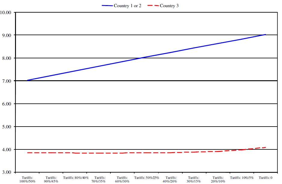
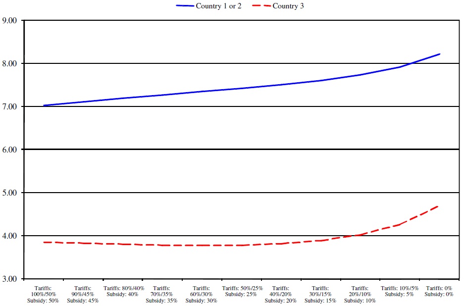
For a trade agreement to be negotiated, the ambitious liberalization schemes must also be in the set of welfare-improving schemes for the two large countries. Individually, the large countries have incentives to distort trade because they have a significant influence on their terms of trade. However, it is well known that in non-cooperative tariff games between two large countries, at most one country wins and both countries are likely to lose (Johnson, 1951; Kennan & Riezman, 1988). A prisoner’s dilemma outcome with both countries worse off at the Nash equilibrium relative to free trade is especially likely when the countries are symmetrical.When this is the case, mandated tariff reductions monotonically increase welfare because the volume of trade increases and the terms of trade remain for the most part unaffected. This is what happens in our simulations with our two large symmetric countries and the DC as shown in Figures 13 and 14. Because large countries do not impose restrictions on the set of feasible multilateral trade agreements and because the restrictions imposed by the DC are such that the set of mutually-beneficial liberalization schemes is not empty, we can hope that an agreement is not only feasible, but that it would bring about significant increases in the volume of trade and in world welfare.

13This argumentwas also verified empirically in a study by ERS (2001). They found that eliminating tariffs would account for most (52%) of the potential increase in the world price whereas domestic subsidies would account for 31% of the total agricultural price impacts of all policies. Although export subsidies can be decomposed as a production subsidy and consumption tax, they account for a relatively small share (13%) of the total price distortions caused by agricultural tariffs and subsidies because they are less popular.

Multilateral negotiations pertaining to agricultural trade liberalization are currently at a crossroads. Developing economies are pressing large policy-active countries to lower their subsidies while pressures to open up borders to trade in agricultural products are meeting resistance from a subset of small and large economies. This paper builds a theoretical model relating changes in trade flows of primary and processed agricultural products to changes in tariffs and domestic support while accounting for NTBs. At the consumer level, processed products are differentiated according to their country of origin while primary agricultural goods are homogeneous from the buyers’ perspective. To account for the notorious NTBs in agriculture, it is assumed that primary goods cannot be substituted costlessly across destinations from the sellers’ perspective. Examples of NTBs include technical and sanitary regulations. These assumptions yield well-behaved import demand functions at the consumer level and export supply functions at the producer level. Imperfect substitution in consumption and production is captured by two structural parameters. The role of these parameters in explaining bilateral trade patterns is investigated through numerical simulations of a three-country international trade model involving vertically-linked products.

The numerical simulations provide insights as to whether it is more important for a developing economy to seek concessions on tariffs or domestic support from large industrialized countries. It is assumed that two identically large countries use import tariffs to restrict trade in primary and processed commodities. Our benchmark is characterized by tariff escalation, a relatively common phenomenon for agricultural products. Like the US and the EU, our large countries also offer coupled domestic support to domestic producers of the primary good. The DC is a free trader in primary and processed agricultural products. When substitutions in consumption and in production are limited due to important NTBs in the upstream sector and strong product differentiation at the consumer level, it is shown that reducing domestic support while holding tariffs fixed actually decreases the DC’s welfare. Under the tariff-only liberalization scenario, welfare initially decreases, but it increases near the end of the process. Free trade is obviously the first-best policy from the world and the DC’s perspective. However, the DC would prefer the status quo over a scenario in which large countries would implement timid tariff cuts, especially if the latterwere accompanied by aggressive cuts in domestic support. Consequently, theDCwould only support an agreement characterized by ambitious tariff cuts. Because our large countries are symmetrical, reducing tariffs increases the volume of trade without affecting very much their terms of trade. Consequently, the welfare of the large countries increases as tariffs are lowered. The implication is that there are many mutually-beneficial trade agreements, but they all call for ambitious reductions in agricultural tariffs.

Even though our model is based on simplifying assumptions, we believe that it provides useful insights regarding the current negotiations. It certainly explains the ambitious market access demands by DCs. It also shows that a modest agreement is acceptable for large countries. Therefore, large countries might try to coerce DCs into supporting a timid agreement by arguing that a succession of timid agreements would be the fastest and surest way to eventually achieve ambitious liberalization. Given that 150 countries are involved in the negotiations, this argument cannot be entirely dismissed, but failure to quickly raisewelfare in developing economies may seriously undermine their convictions about the benefits of multilateral trade negotiations. Sustainedwelfare losses could incite them to negotiate preferential trade agreements or worse to embrace an import-substitution strategy.

Our results showed that NTBs severely reduce the welfare gains arising from tariff and domestic support reductions. NTBs need to be identified to be eventually lowered. As such, it seems most pertinent to measure the NTBs’ parameter for various industries. Because our theoretical model is closely related to standard gravity models, it lends itself to econometric estimation. However, the vertical relationships between primary and processed goods raise particularly challenging issues such as non-linear restrictions across equations and endogeneity. On the theoretical side, the introduction of asymmetries between large countries and ‘types’ of developing economies with different cost and tariff structures should be considered in future research endeavours.