Many retail stores nowadays sell a range of prepared daily food items such as fried meals, cooked food, salad, and sushi. If such daily items are unsold at closing time, they are disposed or reused as ingredients for other items. It is a typical newsvendor problem to find an optimal amount of their initial supply to maximize an expected profit of the day.
Under practical circumstances, it is difficult to estimate demand function for target items accurately. When forecasted demand is more than actual one, retail stores often mark down a sales price to stimulate demand and to reduce the number of unsold items. If the discount pricing is conducted appropriately, it improves the profit of the day. The retail stores decrease disposal cost and might increase the revenue.
The retail stores, however, have to pay attention to the influence of the discount sales on consumers. Consumers’ reference price will be declined when they purchase the products at a discount price. The reference price is a mental price and plays a role as a criterion to recognize whether an asking price is gain or loss. The reduced reference price decreases forthcoming demand sold at a regular price. As a result, a discount sale one day reduces profit in the future. From a viewpoint of profitability, retail stores should determine the clearing discount price carefully with considering its influence on long-term profit.
The reference price is initially proposed as a reference point in the prospect theory by Kahneman and Tversky (1979). The reference price itself is actively researched especially in the area of marketing science. Kalyanaram and Winner (1995) summarized past research with respect to the reference price and mentioned that the reference price is generated by a series of past sales prices. Consumers react differently according to whether the sales price is less or greater than the reference prices of the consumers. The asymmetric reaction is a key concept on behavioral economics well-researched recently.
Our study aims to derive an optimal clearance pricing on daily perishable products to maximize a longterm expected profit. This paper focuses on a single period model as a first step for the long-term optimization. A model is proposed where stochastic demand, stochastic inventory level, which means the amount of unsold items, and consumers’ reference price effect are considered. Greenleaf (1995) proposed a model for the first time to derive an optimal pricing considering the reference price effect and Kopalle
The problem to determine an optimal supply quantity toward uncertain demand is well-known as newsvendor problem. The newsvendor problem is originally studied by Arrow
In this study, an expected profit function is formulated and analyzed mathematically. First, a profit function with deterministic demand and inventory level in a single period model is discussed. The result reveals that the shape of the profit function depends on the consumer' s attitude toward gain and loss, in other words, on whether consumers are loss-neutral (LN), loss-averse (LA), or loss-seeking (LS). Then, the discussed model is extended to treat stochastic demand and inventory level and a sufficient condition is shown to obtain a unique optimal price to maximize an expected profit.
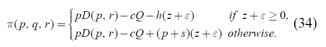
Consider a firm deals in a type of product under monopoly. The target time horizon is limited to a single period in this study. The firm prepares a certain amount of the products before opening time at a unit procurement cost
At a prescheduled time during the operating hours, the firm can discount the products to stimulate demand. This study focuses on the optimal discount pricing. The only decision variable in this model is the discount price
The demand function for the product


The positive parameters
3. OPTIMAL PRICING IN A DETERMINISTIC CONDITION
This section discusses the optimal pricing in case that the demand and inventory level are deterministic as a simple case. In other words, we here treat the case where
3.1 Optimal Pricing for Loss-Neutral Consumers
This subsection confines our discussion to the optimal pricing for LN consumers. Let

The both parameters

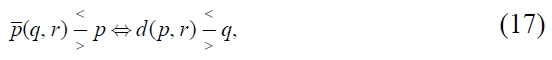
be the price
When the products are sold at price


Let

be the price
Let p* (
Theorem 1:

Proof: The function
Meanwhile, the function
Hence, the profit
where
where
and

exits in [
and monotonically decreases for
Then, the greater between
and
maximizes the profit
Corollary 1:
Proof:
The above inequalities directly derive the corollary. □
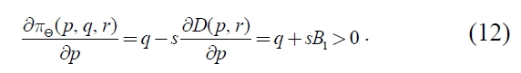
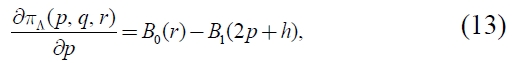
Differentiating
and
with respect to
Hence, both
and
increase monotonically with respect to
is twice that of
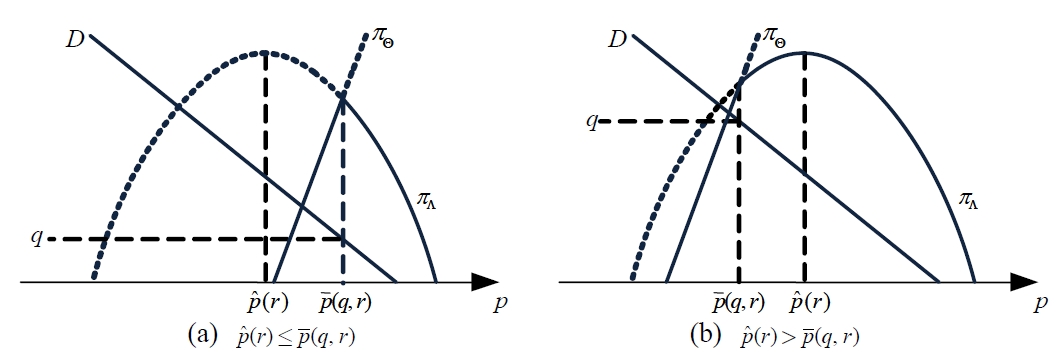
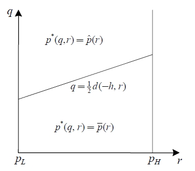
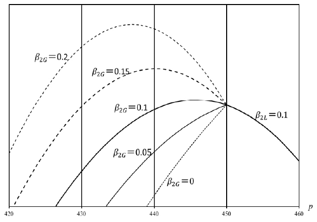
Figure 2 illustrates the region regarding the optimal price with assuming
and
An numerical example for the optimal price
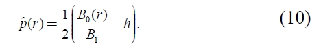
Here, let

be the

then Equation (10) yields
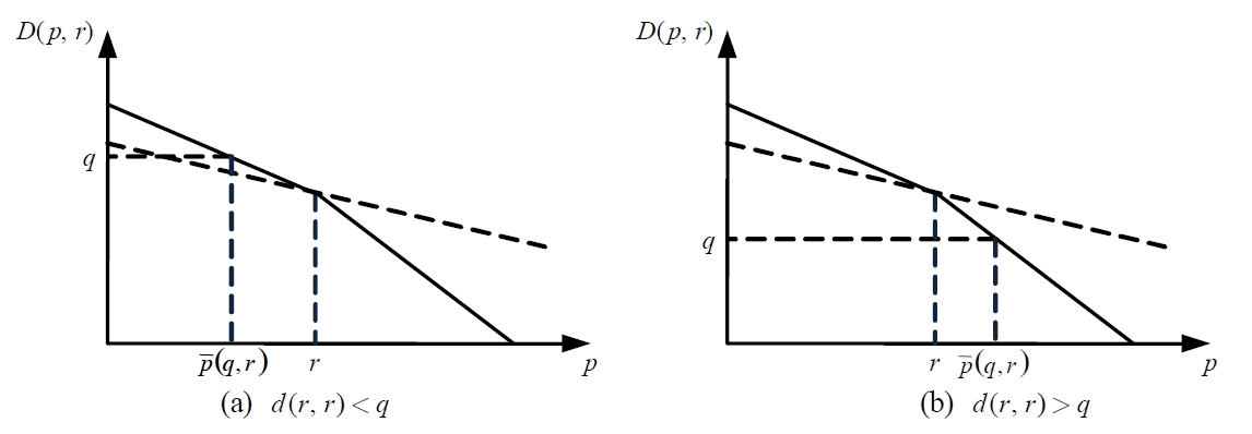
Lemma 1 explains the influence of
Lemma 1:


Proof: Differentiating Equation (10) derives
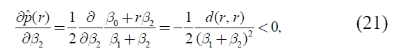
hence
is decreasing with respect to
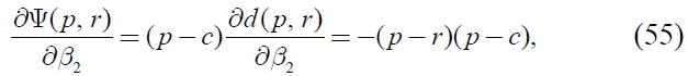
From the assumption that
with respect to
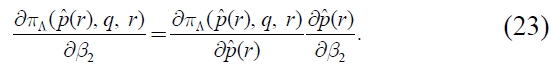
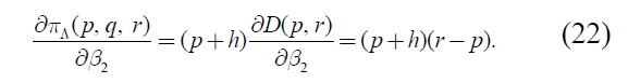
Equations (21), (22), and (23) prove the last property regarding the maximum of profit
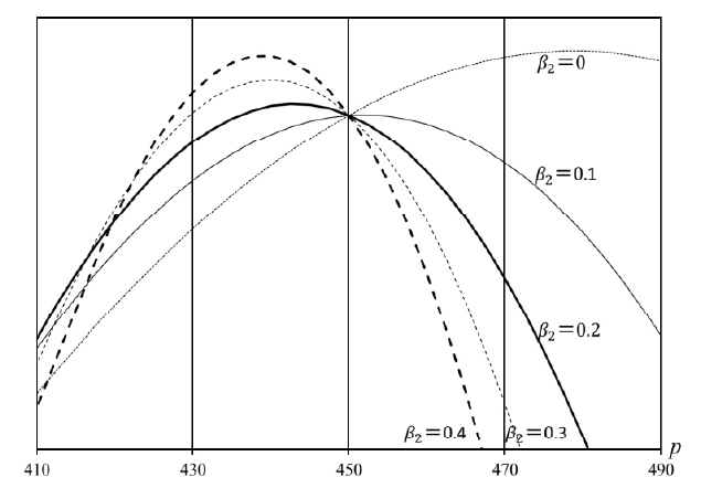
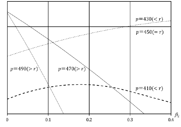
The profit functions

Since
decreases monotonically with respect to
The vertex of

3.2 Optimal Pricing for Asymmetry Consumers
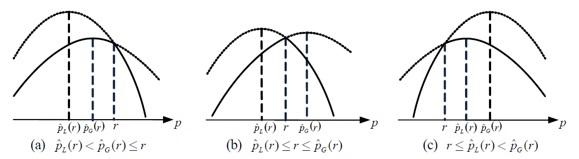
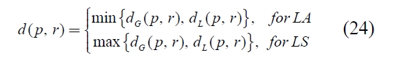
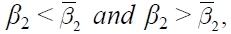
This subsection discusses the optimal pricing for LA and LS consumers, namely when it holds that
since both
In the same manner in the previous subsection, as
was defined as follows:
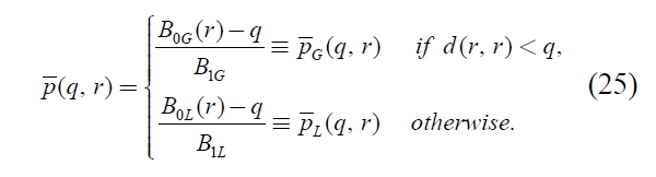
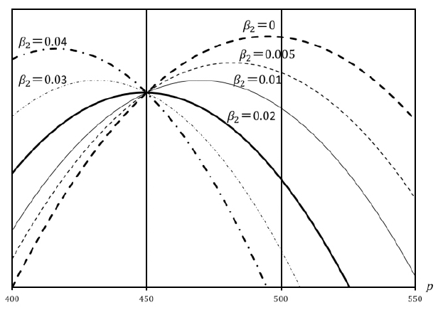
Figure 5 indicates the two prices

and

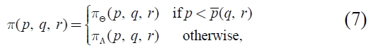
Since Equation (7) also holds for LA and LS consumers,
From Equation (8), the profit function
where
The profit function
since Equation (9) shows

and

be respectively the prices on which
Lemma 1 concludes that it holds
LA consumers and
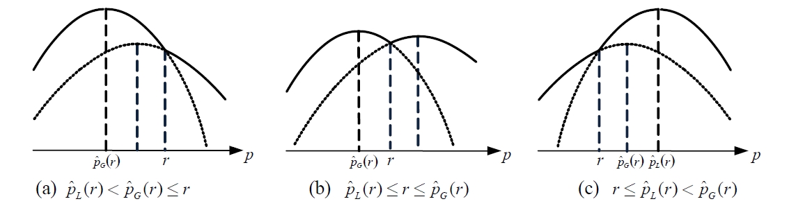
for LS consumers. Then, Lemma 1 restricts the possibility of the shapes of the profit functions
when the function is bimodal. This discussion introduces the following theorem as a procedure to derive the optimal price for the asymmetry consumers.
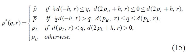
Theorem 2:


Proof: The set
in the middle case in Figure 7,

and

could be optimal. In the case of max
is the optimal price both for LA and LS consumers. Similarly,
is the optimal
when it holds min
In the last case, the middle case in Figure 6,
Note that the cardinality of
In the other cases, the cardinality is one and Equation (32) explores the optimal price without Equation (30).
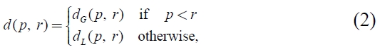
4. OPTIMAL PRICING IN STOCHASTIC CONDITION
This section discusses the optimal pricing in case that the demand
4.1 Optimal Pricing for LN Consumers
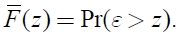
This subsection confines our discussion to the optimal pricing for LN consumers. The demand function
The average of
Let
The expected profit Π(
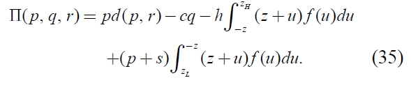
The expected profit Π(


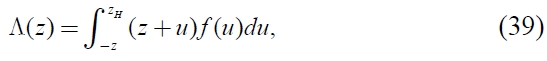
In Equation (36), Ψ(
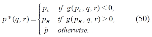
Theorem 3:
where

Proof: Differentiating from Equations (36) to (40) with respect to pyields
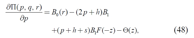
Using the assumption of
which satisfies
Corollary 2:
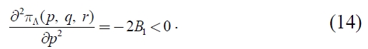
Proof: It is obviously proved from the concavity of the function π(
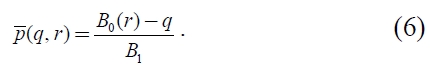
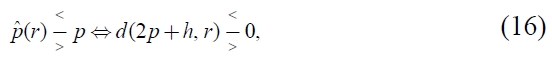
Similarly to the deterministic case, let
be the

then
is obtained from the equation
provided that
is not equal to 0. The next lemma reveals a property on Π (
Lemma 2:

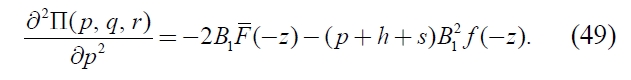
Proof: Differentiating from Equations (36) to (40) with respect to
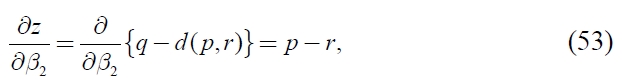
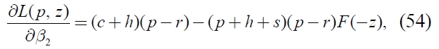
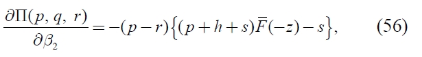
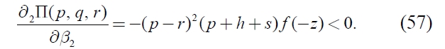
Equation (57) proves the concavity of Π(
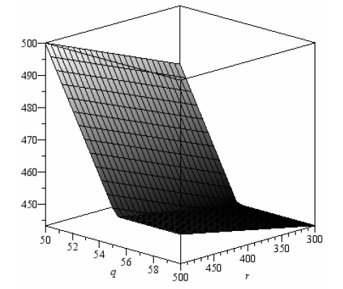
Lemma 2 indicates that the contour of the expected profit function Π(
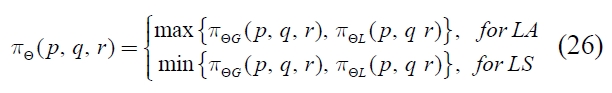
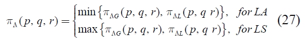
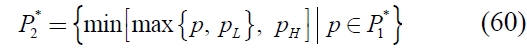
4.2 Optimal Pricing for Asymmetry Consumers
In the case of
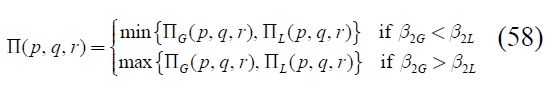
where Π
Similarly to the deterministic case, let

and

be the prices to maximize Π
Theorem 4:

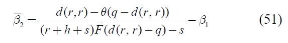
Proof: Differentiating the left hand side of Inequality (52) with respect to
It is noticeable that Inequality (52) can be written as follows:
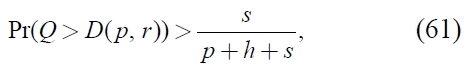
since
Inequality (61) has the same form as the well-known critical fractile for newsvendor problems. It could be practical that the unit penalty cost
In this paper, an optimal clearance pricing in a single period has been discussed analytically considering consumer’ s reference price effect. The profit function in deterministic case is concave if target consumers are LN or LA. For LS consumers, the function is concave or bimodal. In the stochastic case, if Inequality (52) holds for
The resulting theorems in this paper can be applied to the optimal clearance pricing in a multi-period case, which is the goal of our forthcoming study. The model in this paper can be modified to a combinatorial optimization, in which the firm determines the clearance price among several selectable prices, such as 10% off, 20% off, and 50% off. The modified model is more practical and the theorems in this paper could serve to reduce computational time to explore the optimal solutions.