Many OECD(Organization for Economic Co-operation andDevelopment) countries have run government deficits since the mid-1970s. Policymakers experiencing fiscal problems have had to reduce their budget deficits to consolidate government budgets. As a result, in some cases, the public financial position has recovered.
However, once governments implement fiscal adjustments, the size of deficit reductions during periods of fiscal adjustment is not always sufficiently large. For example, the Italian government has implemented fiscal adjustments since 1989. However, Alesina and Perotti (1996) show that the size of the adjustment is much smaller than in other countries analyzed in their study, with the debt to GNP ratio reaching 125% in 1994. Moreover, European countries meeting European Monetary Union entry requirements have had different levels of success in improving their government budget balances.1 The foregoing indicates that even if fiscal authorities attempt to reduce deficits during the fiscal adjustment period, the size of the reductions may sometimes be small.
Differences in the ‘size (or performance)’ of deficit reductions during periods of fiscal adjustment may be due to the differing strength and durability of the government and the budget process. In support of this, Ihori and Itaya (2001) examine the dynamic properties of fiscal reconstruction by a differential game among interest groups. They show that the steady state level of government debt under the Pareto efficient (cooperative) outcome chosen by a benevolent government is smallest among all strategies. In other words, Ihori and Itaya (2001) show that debt accumulation under a benevolent government, which may correspond to a government with strong leadership, is smallest during periods of fiscal adjustment.2 These results suggest that a government with a unified governance structure can reduce budget deficits successfully during periods of fiscal adjustment; whereas a government without numerical targets for the budget balance and procedural rules to be used in the budget negotiation process, or a coalition government, is unlikely to significantly reduce budget deficits.
However, to the best of our knowledge, there has been no rigorous empirical study of the influence of government decision making on the size of deficit reductions during periods of fiscal adjustment. Empirical research on the relationship between fiscal adjustment and the government decision-making process has focused on the credibility of fiscal adjustment, that is, on how sustainable the initial change in the deficit is believed to be among nations. Relevant studies include Tavares (2004), Lavigne (2006), and Mierau
On the other hand, some case studies, such as Alesina and Perotti (1996) and Alesina
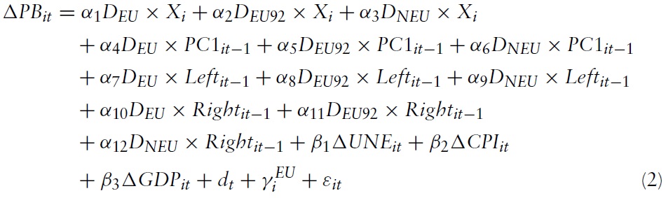
The objective of this paper is to provide empirical evidence regarding the effect of political and budgetary institutional factors on the performance of deficit reductions during fiscal adjustment periods in OECD countries. On the theoretical aspects, the arguments proposed by Ihori and Itaya (2001) imply that the ‘fragmented government,’ which may be a coalition or a government without ‘good’ institutions, tends to be influenced by interest groups and cannot reduce the government’s budget deficits. Hence, ‘fragmentation’ refers to the influence of two factors: political fragmentation is the number of governing parties and their ideologies, and procedural fragmentation refers to numerical targets for government expenditure and procedural rules in the budget negotiation process.3 Our analysis focuses attention on the effects of these two factors and we investigate how they influence deficit reductions during periods of fiscal adjustment.
Incidentally, most of the empirical literature as to fiscal adjustments only deals with political factors and neglects the effect of budgetary institutions. The reason why previous work does not consider the effect of institutions could be that countries with good institutions probably need smaller fiscal adjustments because they may not run large deficits in the first instance. Lavigne (2006) has statistically proven this point. However, on a practical level, countries that have procedural rules for negotiation and numerical targets for government expenditures sometimes suffer fromlarge government deficits that they have to reduce. For example, European countries such as Denmark and Ireland set limits based on numerical targets. However, the public financial condition of Denmark deteriorated rapidly starting in the late 1970s, so that Denmark reached its highest deficit in 1982 and then had to reduce its government budget deficits. In Ireland, although the government has employed specific quantitative targets since the beginning of the 1980s, the fiscal balance continued to deteriorate from the early to mid-1980s, and it needed to launch an adjustment programin 1987 thatwas of different character to the earlier failed program.4 Furthermore, in the UK and Germany, the Prime Minister or Finance Minister strongly influences his or her government’s budget negotiation processes.However, it is difficult for German governments to meet the targets established by the MaastrichtTreaty because fiscal authorities in Germany have had some difficulty in reducing their budget deficits. Among non-European countries, such as Canada and the US, there are limits or targets imposed on ministerial spending before ministers submit their requirements. However, the US suffered from large budget deficits from the mid-1980s to the mid-1990s and the government was obliged to consolidate its budget. During the sample period in this paper, we confirmed that fiscal conditions may sometimes plague countries with good institutions and strong fiscal authorities and this situation requires a reduction in the budget deficit. Hence, we should also consider the effects of institutional arrangements.
The paper is structured as follows. In Section 2, we present an empirical specification and the variables used in the estimation. Section 3 details the empirical strategies and the results. Section 4 concludes.
1See von Hagen et al. (2001) for an analysis of the adjustment experience of individual European Union (EU) member states during the Maastricht convergence process. 2The case of local governments is investigated theoretically in Ihori and Itaya (2004). 3See Perotti (1998) and Perotti and Kontopoulos (2002) for detailed discussion of fragmentation in the fiscal policy decision-making process. 4For a case study of these countries, see Alesina and Perotti (1996). On the fiscal targets in Ireland, see De Haan et al. (1999).
The following set of variables determines budget deficits:

where Δ
From equation (1), the basic regression specification is as follows:
where
For the change in the budget deficit, we use the difference in the cyclically adjusted primary government balance as a ratio of potential GDP, Δ
To reflect country-specific factors in the estimated coefficients, we employ three regional dummies,
We employ institutional index (
The sample period of the indices used in Perotti and Kontopoulos (2002) ends in 1995. In the 1990s, some countries reformed their institutions. In particular, in 1995, Sweden decided to adopt expenditure ceilings, and Australia set limits for annual expenditures based on forward estimates after the Charter of Budget Honesty Act was established in 1998. Because these reforms are related to the issues considered in our study, we exclude these two countries after the first year of institutional reforms when selecting the periods of fiscal adjustment in Section 3. For other reforms, changes to the process are not related to the aspects that we consider here and the trial was temporary.8 In accordance with these features, we use the indices from Perotti and Kontopoulos (2002) and present these in Table 1.
First, we use the variable
[Table 1.] Institutional Indices
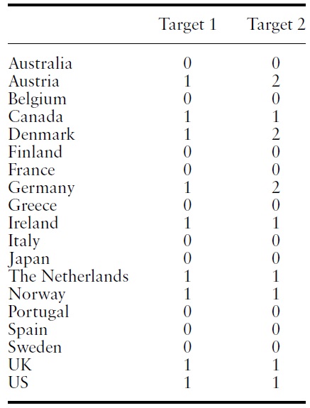
Institutional Indices
Second,
The number of spending ministers may also be specified as another variable to measure the degree of political fragmentation. However, this is less important because institutional arrangementsmay reduce the number and power of spending ministers.9
Δ
5Both our cyclically adjusted primary government balance and potential GDP are taken from the OECD Economic Outlook database. We use cyclically adjusted data because we can identify the outcome of efforts for deficit reduction during periods of fiscal adjustment, while non-cyclically adjusted data contain the improvement of government budget thanks to the economic recovery as well as the efforts for deficit reductions. Then, to make these compatible with the data source of a numerator, we employ the potential GDP as a denominator. Moreover, if we estimate equation (1) by using non-cyclically adjusted government balance to actual GDP as a dependent variable, the results are not favorable in comparison to the ones that we report in the paper. Therefore, in terms of the estimation results, the use of the cyclically adjusted primary government and potential GDP are also recommended. 6Norway has not joined the EU. Therefore, we re-estimate equation (2) by omitting Norway from the DEU92 group but the estimation results are largely unchanged. 7Perotti and Kontopoulos (2002) use the variable ‘NEGOT’, which takes a value of 0 if the negotiations are conducted by the Finance Minister, the Prime Minister or both, and 1 if they are conducted by a committee or the entire cabinet. However, there are no countries in the sample where the entire cabinet actually participates in the budget negotiations. Therefore, we believe it is inappropriate to attempt to measure the power of fiscal authorities and do not employ it as a variable in this paper. 8For example, Japan conducted fiscal reform from 1997 by enforcing the Fiscal Structural Reform Act, but the act was suspended in December 1998. See von Hagen (2006) for a discussion. Further, as mentioned in Perotti and Kontopoulos (2002), the reforms in Belgium and Italy do not relate to the aspects considered here. 9We estimate equation (2) including this variable, but the estimated coefficient is not significant. 10We can use unemployment data because we use cyclically adjusted fiscal data from the OECD, and OECD cyclical adjustment takes into account only movements in GDP, not unemployment. 11We estimate equation (2) by adding outstanding debt to GDP to independent variables. However, the estimated coefficients for this variable are not significant. 12Equation (2) is also assumed to use these variables with a lag to account for the lags from policymakers in response to the economic environment for ΔUNEit and ΔGDPit, and the simultaneity that the budget deficits induce in inflation for ΔCPIit. However, the coefficient estimates for these variables do not change significantly. 13Including all the European country dummieswould involve exact collinearity andmake estimation impossible.We deal with this problem by removing the dummy for the UK. However, changing the reference or omitted category country may change the estimated coefficient on DEU × Xi. To be certain, we re-estimate equation (2) by omitting the dummy variables for other countries in Xi one by one,whilewe include the dummy variable indicating the UK in equation (2). However, the results shown in Table 3 are almost unchanged.
All economic data sets are from the OECD Economic Outlook database.
In our estimation, we restrict the sample to periods when each government implemented fiscal adjustment. From the fiscal adjustment episodes defined in earlier studies, we select the periods during which the budget surplus is positive and lasts several periods in order to specifically reflect the outcome of strong and deliberate efforts by the government for deficit reductions. Thus, a period of fiscal adjustment is defined as the one in which Δ
In a cross-country sample, the specific circumstances of each country (e.g., wars, natural disasters and so on) are more crucial and these factors may sometimes have an excessive influence on the government budget.15 On this basis, including outliers will result in the selection of incorrect periods, even though they are not ‘true’ periods of fiscal adjustment. Therefore, we remove Δ
[Table 2.] Periods of fiscal adjustment
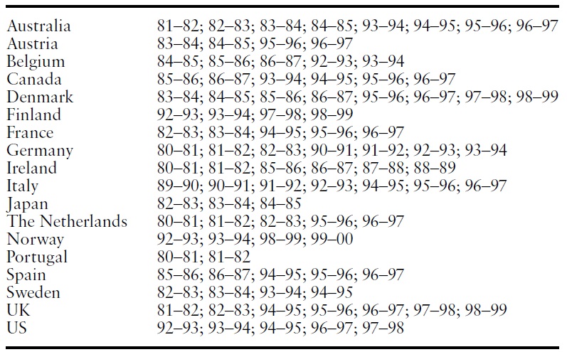
Periods of fiscal adjustment
Here we confirm whether the periods selected encompass actual episodes of fiscal adjustment. First, the episodes for the US in this analysis correspond to the Clinton Administration’s reforms aimed at deficit reduction. The episodes for Ireland in the 1980s involve fiscal reforms centered on the privatization of public enterprises. The reforms referred to as ‘fiscal reconstruction without tax increase’ in Japan in the early 1980s and Canadian fiscal reformafter 1993 are also included in the selected fiscal adjustment periods. From these and other episodes that we examine, it would be fair to say that the selected periods in this paper almost exactly coincide with actual periods of budget deficit reduction during periods of fiscal adjustment.

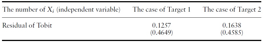
The results of testing selectivity bias. Dependent variables: The change in cyclically adjusted primary government balance (percent of potential GDP). Number of observations = 95.
It is important to note that the data used comprise an incomplete panel because we omit some periods and countries. Moreover, although we assume that the countries implement fiscal adjustment implicitly, the economic conditions and political factors may also influence decision making related to fiscal adjustment, as shown in von Hagen
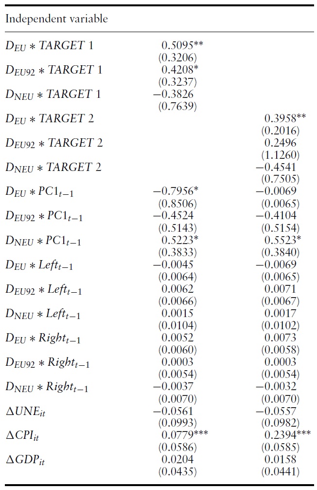
Table 4 reports the results of the least squares estimation. The coefficients of
Incidentally, the estimates of

Estimation results of equation (2) by least squares. Dependent variables: The change in cyclically adjusted primary government balance (percent of potential GDP). Number of observations = 95.
Estimation results of equation (2) by the instrumental variable method of Hausman and Taylor’s (1981) random effects model. Dependent variables: The change in cyclically adjusted primary government balance (percent of potential GDP). Number of observations = 95.
The results of the instrumental variable estimation using the Hausman and Taylor (1981) method are shown in Table 5.21 The estimation results are almost identical to those in Table 4. The coefficients of
14http://www.marquette.edu/polisci/Swank.html 15For example, in the US from 2001 to 2002, ΔPBit decreased by 3.15 percentage points.The events of September 11 and tax reductionsmay haveworsened the government budget.Moreover, in Germany, ΔPBit decreased by 3.3 percentage points from 1989 to 1990 when East and West Germany were reunified. These episodes are judged as outliers by the procedures used in this analysis. 16If we do not remove these data, 112 adjustment episodes are selected. Although we estimate equation (2) based on these 112 episodes, the coefficients of DNEU × PC1t−1 and DEU92 × Rightt−1 are significant. However, the level of significance of the coefficient of DNEU × PC1t−1 is 10%, while it is 5% as shown inTable 3.Therefore, we conclude that the estimation results obtained by including outliers are unfavorable. 17To deal with the fiscal adjustment episodes that one regime carried out, we also examine the cases that were consecutive and conducted by the same regime. Specifically, we select the 74 episodes in which the ideology of the ruling party was the same for two years, determined to be the fiscal adjustment periods. The results are as follows: none of the coefficients of TARGET 1 are estimated significant; for TARGET 2, only the coefficient of DEU × TARGET2 is estimated to be positive and significant. The detailed results can be obtained from the author upon request. 18For more details, see Wooldridge (1995) and Baltagi (2005). 19Detailed results can be obtained from the author upon request. 20Both two-party and PC1t−1 appear to take on very similar values and if we use this variable as an instrumental variable, problems with multicollinearity may arise. However, the correlation may not be strong because two-party involves other countries included in PC1t−1. In fact, the coefficient of correlation is 0.65. Therefore, we can use two-party as an instrument for DNEU × Xi. 21Hausman and Taylor’s (1981) estimation is based on the random effects model. Random effects estimators are more efficient than LSDV estimators (e.g. Baltagi, 2005) . Therefore, compared with the results shown in Table 4, standard errors in Table 5 tend to be smaller. 22To check the effects of political factors, we re-estimate equation (2) by multiplying PCit−1 by Leftit−1 and Rightit−1. For the political variables, only the coefficient of Left × PC1it−1 in non-European countries is found to be positive and significant. This may reflect the fact that most of the episodes in non-European countries were fiscal reforms completed under left governing parties, such as the Democrats in the US and the Labor Party in Australia. For another test of robustness, we re-estimate equation (2) by specifying the dependent variable in levels. However, if we estimate the cyclically adjusted primary government balance as a ratio of potential GDP in levels, the coefficients of the Tobit residuals are significant and we reject the null that there is no selectivity bias. Detailed results can be obtained from the author upon request.
This paper investigates how both political factors and budgetary institutions influence the size (or performance) of deficit reductions during periods of fiscal adjustment. For all cases, our empirical findings using OECD data indicate that while countries with a fiscal target are likely to reduce their budget deficits successfully at a time of fiscal adjustment in Europe, the political leadership of a single-party government is the key determinant of fiscal adjustment in non-European countries.
Our results show that countries with a fiscal target reduce budget deficits successfully when the government makes genuine efforts to restore fiscal conditions. In fact, even countries with a fiscal target had to cut budget deficits or expenditures for several years in order to meet their target values. Reflecting this point, the results may also suggest that the set of fiscal targets is effective in supporting temporal efforts for deficit reduction. Above all, in European countries, the effect of a fiscal target is robustly confirmed in all estimations. Many earlier studies of budgetary institutions in European countries have shown that the effectiveness of fiscal rules or the strength of fiscal authorities depends on the political environment. 23 Contrary to the earlier works, our findings show that fiscal target is effective in deficit reductions during periods of fiscal adjustment from the 1980s to the early 2000s, regardless of political factors.
On the other hand, for non-European countries in our sample (Australia, Canada, Japan, and the US)we demonstrate that the government could reduce the budget deficits successfully during the periods of fiscal adjustments. Compared with most European countries, these countries do not tend to have coalition governments. Hence, the strong leadership of a single-party government may be strongly confirmed.
Incidentally, to maintain consistency with Ihori and Itaya’s (2001) theoretical hypothesis, we consider both political and institutional factors here. However, another factor such as the potential role of election years (upcoming elections) and the possibility of broad policy reformmight also affect the size of fiscal adjustments. Moreover, in selecting the periods of fiscal adjustment, it is necessary to choose periods based on ‘successful’ fiscal adjustment episodes. This procedure allows us to investigate the relationship between the attributes of fiscal adjustment and political or institutional factors. Finally, for institutional indices, recent studies such as IMF (1998), OECD (2001), and Alt and Lassen (2006) develop a ‘transparency index.’ We may then need to analyze further the issues arising in this paper in terms of fiscal transparency. Future work should deal with these interesting extensions.
23For example, see von Hagen and Harden (1995), Hallerberg and von Hagen (1999), and von Hagen et al. (2001).