A comprehensive understanding of atmospheric parameters like wind and temperature on small (<100 km) to global scales for all times of day are crucial to research the principle of Earth’s climate, and to prevent meteorological disaster [1-13]. Rayleigh Lidar detects atmospheric parameters by transmitting laser to the atmosphere and receiving the backscattering signals from molecules. The Rayleigh cross-sections follow a
Based on the former Doppler Wind Lidar (DWL) of University of Science and Technology of China (USTC), a new mobile Rayleigh Doppler Lidar and a new scanning Rayleigh Doppler Lidar for wind and temperature measurements in the stratosphere and lower mesosphere were developed by USTC and the results werereported in 2014 and 2018 respectively [11-15]. But the wind and temperature results of the stratosphere and lower mesosphere during daytime were rarely reported.
In this paper, in order to obtain the wind and temperature data of the stratosphere and lower mesosphere in daytime, an ultra-narrow bandwidth filter (UNBF) matching the double-edge technique of former Raleigh Lidar of USTC has been developed. The improvements of SNR of Raleigh Lidar working in daytime are shown and the results are presented in this article.
2.1. Description of the Method
The main problem for Rayleigh Lidar worked in daytime is how to restrict the sky background under sunlit conditions. Methods to improve the SNR and to increase the detecting range must be implemented. The total photon counts,

where E0 is the transmitting energy, h and v are Planck,s constant and the laser frequency respectively,
The photon counts of the background light received by the lidar can be expressed as:

where
Because Rayleigh Lidar uses a high sensitivity photomultiplier as the detector and uses photon counting technology for signal receiving, considering the shot noise limit (SNL), the SNR can be calculated by [16, 19, 25]:

where
As can be seen from Eq. (4), a higher SNR needs a larger
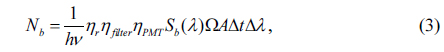
[TABLE 1.] Specifications of the Rayleigh lidar

Specifications of the Rayleigh lidar
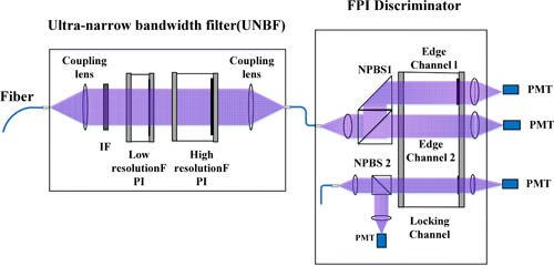
Based on the former DWL system of the USTC, an ultranarrow band filter (UNBF) is developed for Rayleigh Lidar in order to achieve the wind and temperature measurement of stratosphere and lower mesosphere. The parameter design of UNBF is based on the FPI discriminator which adopts a double edge technique with three-channels. The optical structure of FPI discriminator and the UNBF are shown in Fig. 1. The parameters of the FPI discriminator are shown in Table 2. And the parameters of each optical component of the UNBF are shown in Table 3.
[TABLE 2.] Parameters of FPI discriminator
Parameters of FPI discriminator
[TABLE 3.] Parameters of IF and cascaded FPIs
Parameters of IF and cascaded FPIs
As is shown in Fig. 1, the returned signal collected by the telescope is coupled into the signal fiber, and at the other port of this fiber the signal light is changed into a parallel beam by a collimating lens and then enters the UNBF. The UNBF is mainly composed of two coupling lenses, an IF, a low resolution FPI and a high resolution FPI.
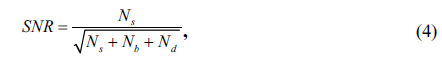
The principle of UNBF design is as follows. Based on the theory that the bandwidth of FPI transmission is narrow, we adopt two FPIs of different resolution which are cascaded with the IF, so a single narrow bandwidth transmittance in the entire bandwidth range of the IF can be obtained for maximum suppression of solar background in daytime. The principle of spectrum of UNBF is shown in Fig. 2(a).
The UNBF is designed based on the double edge FPI discriminator of the USTC. The bandwidth of high resolution FPI is designed by 2 pm (5.1 GHz) according to the edge separation of the FPI discriminator (5.1 GHz). As can be seen from Fig. 2(a) the higher the fineness the smaller the numbers of peak transmission. But the fineness of high resolution FPI is up to 17 based on the existing manufacturing accuracy, so the FSR of high resolution FPI is up to the maximum 34 pm (81 GHz). At this time, there are still more than 4 peak transmissions of high resolution FPI in the bandwidth of the IF. Based on the bandwidth of the IF, a low resolution FPI is designed with FSR of 150 pm and fineness of 17 to insure that there is only a single transmission in the bandwidth of the IF. The spectrum principle of double edge FPI discriminator is shown in Fig. 2(b). Theoretical transmission equation of the FPI is as follows [20-24].

where
Using Eq. (1) to Eq. (5), we can figure out the SNR with-IF and that with-UNBF during daytime. The results are shown in Fig. 3. It can be seen from the simulation results that the SNR of with-UNBF is much higher than the one with-IF during daytime. So Rayleigh lidar with-UNBF could greatly improve the detection altitude during daytime in theory.
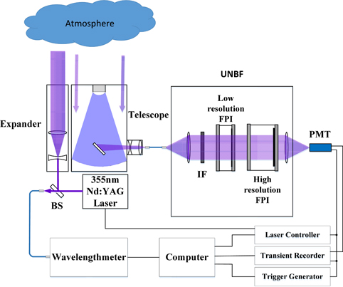
The major system parameters are shown in Table 1 and the schematic diagram of the transmitting and receiving subsystems are shown in Fig. 4. The transmitting subsystem consists mainly of a laser of 355 nm and an expander. The output laser is split into two beams by a beam splitter (BS). One of the output beams is collimated by the expander and transmitted into the atmosphere. The other beam of the 355 nm output laser is coupled into a wavelength meter to monitor the wavelength of the laser by use of a single-mode fiber. The laser wavelength is stabilized by laser controller. The pulse laser, operating at a repetition rate of 50 Hz, has a linewidth of 200 MHz and pulse energy of 350 mJ. The far-field full-angle divergence of the laser is compressed from 0.5 mrad to 30.33 urad via a 15X beam expander.
During the daytime observation, the backscattering light signal is received by a telescope with 1 m aperture, and goes through a battery of collimating lenses where the IF could be inserted and removed freely. Then the signal light passes through the UNBF and is received by a photon counting mode PMT. Last, the data from the PMT is collected by the transient recorder with a range resolution of 7.5 m for the detection from 25 km to 50 km.
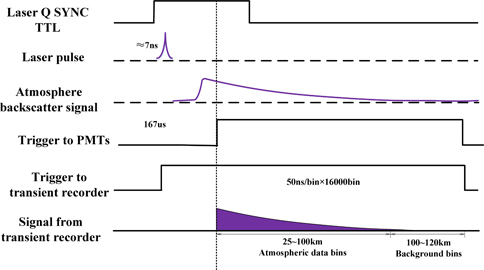
It is useful to step through the timing sequence for a single laser pulse to understand how the signals are collected, as is depicted in Fig. 5. The detector is successfully employed for the data acquisition triggered by a high level of transistor-transistor logic (TTL) from programmable range-gating electronics. The SYNC TTL signal from the laser was used to synchronize the range-gating electronics. In order to prevent the detector from saturating and to receive the signal above 25 km, the trigger generates a low level of transistor-transistor logic (TTL) output during the Q switch to the light reaching the altitude of 25 km. The tail of atmosphere backscatter within the altitude range from 100 to 120 km is used as the average background. The final output data from the transient recorder is shown in Fig. 5. All the sequence is controlled by industrial personal computer (IPC).
III. CHARACTERIZATION OF THE SYSTEM CALIBRATION
In order to receive the returned signal of stratosphere and lower mesosphere with high SNR during daytime, the transmission curves of the two FPIs should be calibrated to ensure that the measured parameters are as consistent as possible with the designed parameters.
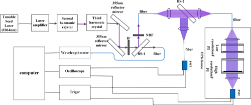
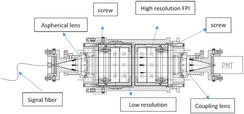
Figure 6 gives the schematic view of the optical setup for the calibration experiment of UNBF transmission. The experiments are carried out in a dark laboratory environment because of the extreme sensitivity of the PMT for photons, with environment temperature stabilized by an air-conditioning system. The tunable seed laser injects the laser amplifier by a single mode fiber, and the amplifier emits pulse laser which is converted into 355 nm pulse laser by the second harmonic crystal and the third harmonic crystal. The 355 nm pulse laser passes through an IF by two 355 nm reflector mirrors and is split into two beams by the beam splitter-1 (BS-1). The transmitted beam is coupled into a single mode fiber connected with wavelength meter which is used for monitoring the actual wavelength of the emitted laser. The reflected light passes through a neutral density filter (NDF) which is used for reducing the incident light because the PMT is working in the mode of single photon counting. Then the reflected light is collimated by a lens and split by BS-2. The light reflected by BS-2 is coupled into a fiber and received by a PMT. The transmitted light is coupled into a fiber and collimated by an aspherical lens and then enters the FPIs’ housing at normal incidence. The structure of FPIs’ house is shown in Fig. 7 and the splitting ratio of BS-2 is measured before the experiment. Finally the light passing through FPIs housing is coupled into the other PMT. The timing sequence of data acquisition is controlled by trigger and the data is acquired by oscilloscope. All of althe electronic devices are controlled by a computer.
To make sure that the two cascaded FPIs work at the same central wavelength, the experimental process is divided into two steps. In the first step, the transmittance curve of each of the two FPIs should be calibrated with the experimental system. During this experimental process, there is only one FPI in the FPI’s housing. Keeping the wavelength of incident light fixed, the central wavelength of a single FPI should be kept consistent with incident light by adjusting the screws shown in Fig. 7. The screws are made of invar to make the FPI be stabilized at different ambient temperatures. When the experiment is finished, take out the calibrated FPI and install the other FPI for calibration by the same technique. In the second step, the two FPIs are installed in the FPIs’ housing as is shown in Fig. 7 and then the actual transmittance curve of cascaded FPIs is measured. In this step, the wavelength of incident light is the same with the first step. During all the experiments, the light strikes the PFIs at normal incidence.
3.1. Transmission Curve of Each FPI
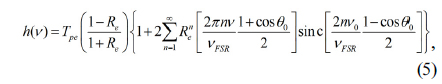
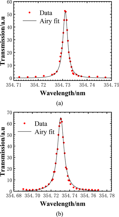
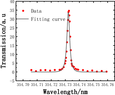
The transmission curves of a single FPI and the cascaded transmission curves of two FPIs of UNBF are tested by a tunable laser. Figure 8 shows the tested and the fitting results of the single FPI. Figure 8(a) shows the result of the transmission curve of the low resolution FPI and Fig. 8(b) shows the transmission curve of the high resolution FPI. The red symbols are the resultant data and the solid lines (black) are the fitting results using the theoretical transmission equation of the FPI in Eq. (5).
According to the fitted results, the measured bandwidth of the high resolution FPI is 2.27 pm, slightly larger than the design value, the central wavelength is 354.73118 nm, and the peak transmission is 52.03%. The measured bandwidth of the low resolution FPI is 8.36 pm, slightly less than the design value, the central wavelength is 354.73004 nm, and the peak transmission is 65.14%. The central wavelengths of the two FPIs basically coincide with a slight deviation of 1.14 pm. From the above measured results, we can see that the test results of a single FPI’s parameters are well matching with the design values.
3.2. Transmission Curve of Cascaded FPIs
Based on the above work, the performance of the two cascaded FPIs was tested. Figure 9 shows the tested and the fitting results when the two FPIs are in the cascaded state. The red symbols are the resultant data and the solid line (black) is the fitting result using the approximate transmission equation of the FPI as follows.
where
According to the fitted results, the measured bandwidth of the cascaded FPIs is 2.4 pm, slightly larger than the design value, the central wavelength is 354.73109 nm, and the peak transmission is 33.71%. Figure 9 shows that the test results of the cascaded FPIs’ parameters are well matched with the design values. Furthermore, the measured bandwidth is slightly larger than the designed value by 0.3 pm, and the main reasons are that the actual parameters of a single FPI deviate from the designed value, especially that the bandwidth of high-resolution FPI is 2.27 pm, which is larger than the designed value. Meanwhile the structure system is not stable enough, the parameters of each FPI would vary slightly in the process of alignment. In addition, the relative position of the cascaded FPIs is not strictly parallel in the process of aligning. All the above factors lead to the measured results being slightly larger than the designed bandwidth.
At the same time, the matching error of the two FPIs, relative position error of two FPIs in the structure system and the measured peak transmission of a single FPI are all slightly inconsistent with the theoretical value. All of the above factors result in the measured peak transmission of cascaded FPIs being slightly lower than the designed value.
IV. CHARACTERIZATION OF SOLAR BACKGROUND RESTRICTION
The UNBF is designed for Rayleigh lidar which is used for detecting atmospheric parameters like wind speed and temperature of stratosphere and lower mesosphere based on the principle of Rayleigh-scattering. On cloudy days, foggy days or rainy days, the pulse laser energy attenuated severely over a long distance, the laser energy reaching the detection altitude is extremely weak or even could not reach the altitude. In addition, aerosols signals would interfere with the measured accuracy of Rayleigh signals. Considering the above conditions, the PMTs are not responding to the aerosols signals by setting the sequence of PMTs delaying 167 us when the laser emits, as is shown in Fig. 5.
In order to achieve the detection for the stratosphere and lower mesosphere, Rayleigh Lidar usually works in sunny weather. Meanwhile, solar background radiation is higher on sunny days than that on cloudy days or on rainy days, so it is better to carry out the experiment on a clear day to compare the background attenuation effect from with-UNBF and with-IF.
Therefore, the below experiments were taken in clear and stable weather in Hefei (32o N, 117o E), southeast of China. The experiment for with-IF and with-UNBF were alternately carried out by one lidar system with the same configurations. It is assumed that all the circumstances like sun-zenith angle have the same impact on the experimental result.
4.1. Solar Background Restriction Analysis
The background level with-IF and with-UNBF are evaluated without laser emission during clear and stable weather in Hefei from 5:00 a.m to 6:00 p.m on 26 August, 2018. In this experiment, we take Licel TR-20-160 as the signal acquisition card with the maximum photon counting rate 250 MHz and accumulation time 5 min.
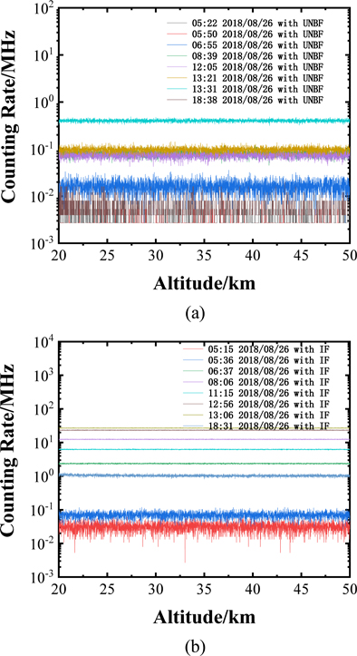
Figures 10(a) and 10(b) show the results of variation trend of the background from early morning to nightfall by with-IF and with-UNBF, respectively. As the sky-background intensity is total background photons in the visual angle of the telescope, so the photon counting rate of sky-background intensity is a constant with altitude in the accumulation time.
Figure 10(a) shows the measured intensity of solar background with-UNBF from 5:00 a.m to 6:00 p.m on 26 August, 2018. The average values are 7.966*10-4 MHz, 0.0154 MHz, 0.0809 MHz, 0.0503 MHz, 0.0808 MHz, 0.0966 MHz, 0.425 MHz, and 0.086 MHz respectively. Figure 10(b) shows the measured intensity of solar background with-IF over the same period on 26 August, 2018. The average value are 0.0313 MHz, 0.0762 MHz, 2.237 MHz, 12.431 MHz, 6.103 MHz, 23.865 MHz, 26.869 MHz, 10.405 MHz, and 12.431 MHz respectively. We can qualitatively see that the solar background with-UNBF is lower than that with-IF.
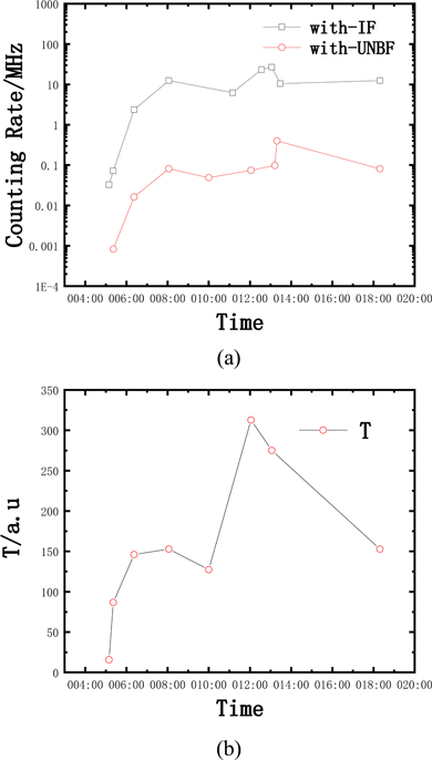
In order to evaluate the performance of UNBF quantitatively, the measured intensity of solar background at different times was averaged and the results were shown in Fig. 11(a). An evaluation function was defined as follows.

where
From Fig. 11(a) we can see that the radiation intensity of solar background is from low to high and up to the maximum, then down again as a function of time. The maximum value of the background happened at about 13:00 pm because of the telescope pointing approximately at the sun. And the solar background with-IF is much higher than that with-UNBF. Figure 11(b) shows the variation trend of T values based on Fig. 11(a). It can be seen that the suppression of UNBF for solar background is 10~320 times higher than that of IF. From early morning to late afternoon, the T values first rose and then fell, and reached the maximum at about 13:00 p.m. So the stronger the solar background, the better the inhibition effect to the solar background. There is a large variation of T value at about 13:00. In my opinion, the sky background light is multispectral and the intensity of radiation around 354.7310 nm (the central wavelength of UNBF) is different at different wavelengths and changes over time.
4.2. Signal Receiving and Analysis in Daytime
In order to precisely make the laser wavelength consistent with the center wavelength of UNBF tested in part 3, the spectral channel uses a wavelength meter to continuously monitor the transmission light and to feed back the result to the computer to control the laser controller. It is shown in Fig. 4.
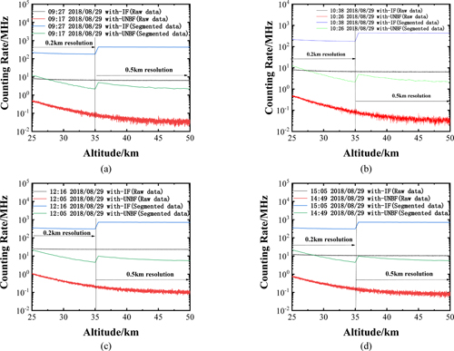
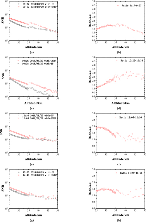
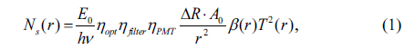
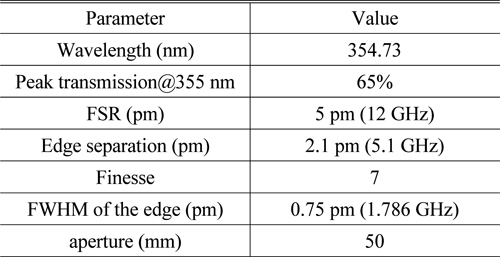
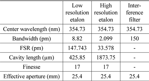
We analyse the lidar SNR according to the returned signal. In order to illustrate the effect of background suppressing of UNBF and that of IF, we choose returned signals in four periods with different background intensities during daytime. The signal is received by with-IF and by with-UNBF during clear and stable weather in Hefei from 9:17 to 9:27, 10:26 to 10:38, 12:05 to 12:16 and 14:49 to 15:05 on 29 August, 2018. The raw data is represented in Fig. 12.
The raw Rayleigh backscattering signal was indicated as a black line with-IF and as a red line with-UNBF. The resolution of the raw signal is 7.5 m. The green curve and blue curve are the segmented signal with the 0.2 km (from 25 km to 35 km) and 0.5 km resolution (from 35 km to 50 km). The blue one is with-IF and the green one is with-UNBF. Accumulation time of the profiles is 5 min. It is shown in Fig. 12(a) that the segmented signal is unable to distinguish up to about 30 km altitude with-IF and to about 47 km altitude with-UNBF from 9:17 to 9:27. Figure 12(b) shows that the segmented signal is unable to distinguish up to about 35 km altitude with-IF and to about 45 km altitude with- UNBF from 10:26 to 10:38. Figure 12(c) shows that the segmented signal is unable to distinguish up to about 30 km altitude with-IF and to about 40 km altitude with- UNBF from 12:05 to 12:16. And Fig. 12(d) shows that the segmented signal is unable to distinguish up to about 30 km altitude with-IF and to about 40 km altitude with- UNBF from 14:49 to 15:05.
Then we can see qualitatively that the returned lidar signal was buried in the background noise at the altitude about 25 to 30 km with-IF and about 45 to 50 km with-UNBF respectively. So the detecting distance of Rayleigh Lidar has been improved with-UNBF.
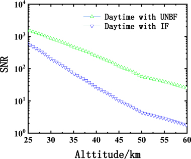
For further quantitative analysis, it is necessary to discuss the SNR of different altitudes. The SNR is defined as Eq. (4). Figs. 13(a), 13(c), 13(e) and 13(g) show the SNR of the returned signal received from 9:17 to 9:27, 10:26 to 10:38, 12:05 to 12:16 and 14:49 to 15:05 with-IF and with-UNBF respectively. The black point plot indicates the SNR with-IF and the red point plot indicates the SNR with-UNBF during the same period.
Figures 13(a) and 13(c) show the results at morning and forenoon respectively. We can see that the SNR with-UNBF has a certain improvement effect in general compared with-IF from 25 km to 50 km. The SNR with-UNBF and with-IF in Fig. 13(a) are from 5193.19 to 1645.47 and from 3557.44 to 913.99, respectively, in the altitude range, 25~35 km. From 35 km to 50 km, the SNR with-UNBF and with-IF are from 2376.36 to 382.65 and from 1161.86 to 498.29, respectively, in Fig. 13(a). In Fig. 13(c), the SNR with-UNBF and with-IF are from 2830.71 to 809.84 and from 2596.75 to 289.37, respectively, from 25 km to 35 km. From 35 km to 50 km, the SNR with-UNBF and with-IF are from 1194.13 to 215.91 and from 497.89 to 122.46, respectively, in Fig. 13(c).
Figures 13(e) and 13(g) show the results at noon and afternoon respectively. We can see that the SNR with-UNBF has a certain improvement effect in general compared to with-IF from 25 km to about 40 km and from 40 km to 50 km they are similar because the wavelength of laser drifts slowly and is inconsistent with the central wavelength of UNBF, so the returned signal is lower than that where the wavelength of the laser is consistent with the central wavelength of UNBF and SNR with-UNBF is lower. The values of SNR with-UNBF are from 5012.19 to 843.19 and from 2649.54 to 845.35 with-IF, in Fig. 13(e). In Fig. 13(g), the values of SNR with-UNBF are from 4231.19 to 586.97 and from 3157.69 to 543.1 with-IF.
The ratio of with-UNBF SNR to with-IF SNR are calculated according to Eq. (8).

where
The values of Ratio are shown in Figs. 13(b), 13(d), 13(f) and 13(h) at different periods. As can be seen from Fig. 13(b), the values of Ratio are larger than 1 from 25 km to 45 km and reach the maximum 2.2 at 36 km altitude at 9:17 to 9:27. And at 10:26 to 10:38, the Ratio values are larger than 1 from 25 km to 50 km, it reaches the maximum by 3 at 40 km. In my opinion, the reason is that the wavelength of the laser drifts slowly versus time, and it is close to the central wavelength of the UNBF at this moment, so the SNR with-UNBF is much higher at this moment. In the afternoon, the Ratio values are larger than 1 from 25 km to 40 km at 12:05 to 12:16 and at 14:49 to 15:05. From 40 km to 50 km, the Ratio values fluctuated around 1. Because at this time, the actual difference between wavelength of the laser and central wavelength of the UNBF is becoming larger versus time, so the SNR with-UNBF decreases compared with the SNR of with-IF and the Ratio-values decrease accordingly.
In conclusion, the SNR with-UNBF could improve by 3 times from 35 km to 40 km at 10:26 to 10:38 on August 29, 2018 in this experiment. And the comparison result shows the SNR with-UNBF is better than that with-IF for Rayleigh Lidar system during daytime in a certain range of altitude. The SNR can be increased by 1 to 3 times versus altitude in general. The ongoing study will concentrate on how to keep the wavelength of laser and the central wavelength of UNBF the same over time.
The goal of this work is to develop an ultra-narrow bandwidth filter and to measure the lidar backscattering signal at the wavelength of 355 nm, making the photon counting technique possible in daytime. This is the first time, to our knowledge, that the cascaded FPIs with IF are used for returned signal detection of the lower mesosphere and stratosphere in daytime. The prototype of the UNBF represents a viable option to restrict strong solar background for an operational lidar designed to measure the atmosphere parameters of lower mesosphere and stratosphere during daytime. The experiment detects the returned signals from 25 to 50 km and the analysis illustrates that the SNR was improved by 1~3 times at this altitude range. However, the stability of the prototype would be improved because the UNBF was affected easily by the environmental factors such as temperature and vibration. Meanwhile, measurements should be introduced to inhibit the frequency drift of the laser.
The idea and primary experiments in this paper present a possible solution to the operational observation problems normally associated with photon counting Raleigh Lidar. In Fig. 4, the PMT at the end of the UNBF could be replaced by an FPI discriminator to measure the variation of Doppler frequency and realize the wind speed measurement for the stratosphere and lower mesosphere during daytime.