In recent years, quantum technology has flourished and quantum imaging technology has developed.
As a new imaging method, associative imaging has attracted wide attention in the field of image transmission [1-9]. Ghost-imaging techniques continue to evolve, from entangled photon pair [1] to thermal sources [2], from traditional ghost imaging to computational ghost imaging (CGI) [3], and many improved methods such as compressed sensing (CS) [4] and differential correlation imaging [5] have also been proposed. With the improvement of image quality, the influence of turbulence on imaging has attracted more and more attention. In reference [6], a random phase screen was applied to simulate the phase disturbance of turbulence. In reference [7], a thermo-optical ghost-imaging experiment was carried out to verify that it is turbulence-free. In reference [10], the visibility and quality of the ghost image through monostatic turbulence and bistatic turbulence were discussed. In reference [11], numerical calculations to demonstrate atmospheric effects on ghost imaging of a double slit were studied. In reference [12], the spatial resolution, image contrast, and SNR were calculated for ghost imaging through turbulence on rough-surfaced targets. However, the above references rarely research the intensity fluctuation brought by turbulence in a system for compressed-sensing computational ghost imaging (CSCGI).
A variety of intensity-fluctuation turbulence channel models,
The rest of this paper is organized into three sections: The theories of CSCGI and atmospheric turbulence channel are expressed in Sections 2.1 and 2.2 respectively. Then, the scheme for the CSCGI system under GG atmospheric turbulence channel is discussed in Section 2.3. Accordingly, in Section III, PSNR and BER are simulated to measure the performance of the proposed scheme. The PSNR and BER performance are determined by the refractive-index structure parameter , the transmission distance
II. THEORETICAL ANALYSIS AND SCHEME DESCRIPTION
2.1. Theory of Compressed-sensing Computational Ghost Imaging
Ghost imaging, also known as correlated imaging or two-photon imaging, is a quantum or classical correlation feature based on light-field fluctuations. By measuring the intensity correlation function between the reference light field and the target-detection light field, a novel imaging technique that acquires target image information nonlocally is achieved. Correlated imaging is different from general, classical optical imaging, and can be independent of the speed of light; this is an important feature that distinguishes quantum optics from classical theory. It is a new type of imaging technology, but image resolution and contrast are still the most important technical objectives.
Traditional correlation imaging requires two optical paths, causing problems such as experimental difficulties and occupying a large space. To solve these problems, Shapiro proposed computational ghost imaging (CGI) [18], and Bromberg
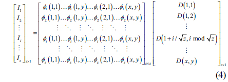
While the computational ghost imaging is running, a series of random modulation matrices

Here 〈
To improve the quality of the reconstructed image, various algorithms are introduced on the basis of ghost imaging, and compressed sensing is one of them. Compressed sensing, also known as compressed sampling or sparse sampling, is a technique for finding sparse solutions for underdetermined linear systems. Compressed-sensing theory utilizes the sparse characteristics of the signal, and the amount of effective information required is much less than the sampling amount required by the Nyquist sampling theorem, which reduces the amount of information collected, saves signal acquisition time, and still reconstructs high-precision images. Low sampling and high reconstruction have been achieved. Combining compressed sensing and ghost imaging, the number of samples has been effectively reduced and the quality of image reconstruction have been effectively improved [21].
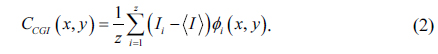
The formula for compressed sensing is:

In computational ghost imaging, the intensity
2.2. Theory of Atmospheric Turbulence Channel Model
The upper atmosphere’s pressure and temperature are affected by wind and other factors. Accordingly, the refractive index of an optical path varies, and atmospheric turbulence occurs. This turbulence results in intensity fluctuations of the received signal, and increases the BER.
There are two methods to simulate turbulence: The first method is to study the effect of atmospheric turbulence on light intensity,
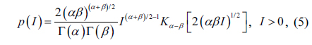
In ghost imaging, there is a bucket detector receiving the total intensity of the transmission image, while the resolution and phase of each pixel in the image is not mainly a concern. As a result, we apply the first method, namely the distribution model, to simulate turbulence. The log-normal and gamma-gamma models are classical models to describe light-intensity distribution. The former is valid for weak turbulence, while the gamma-gamma distribution could be a better choice for a broad range of turbulences(from weak to strong), because both large-scale and small-scale intensity fluctuations can be approximated by gamma distributions.
The gamma-gamma distribution is as follows [17]:
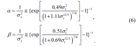
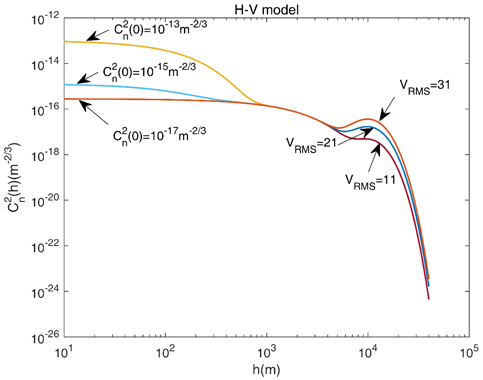
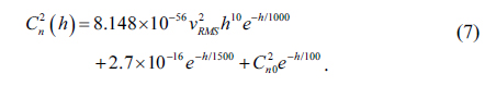
In Eq. (6), and is the refractive-index structure parameter. The degree of atmospheric refractive-index fluctuation is measured by , which varies with altitude and wind speed. In the ITU (International Telecommunication Union) -R H-V model, the relationship between and altitude
It can be seen from Fig. 2 that is approximately invariant with
In this paper, transmission in the horizontal path is researched, so is practically constant. The values of for the different turbulence regimes are as follows:
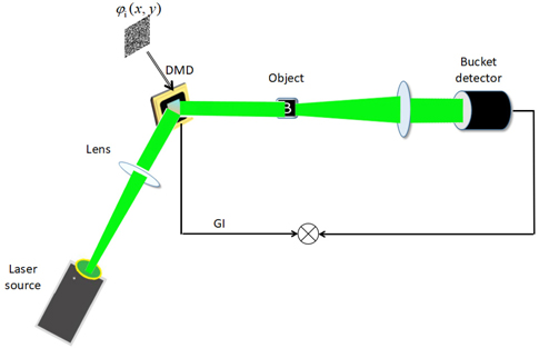
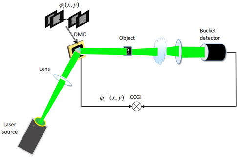
A schematic diagram of image transmission in compressed-sensing computational ghost imaging with the added turbulence model is shown in Fig. 3. After being modulated by the modulation matrix
The received light intensity is obtained from Eq. (8), considering the gamma-gamma turbulence in Eq. (5):

Here
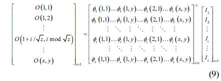
Next we bring the turbulence receiving function of the bucket detector into the compressed-sensing computational ghost imaging of Eqs. (4) and (8) to get the intensity array of the reconstructed image, as shown in Eq. (9):

Here
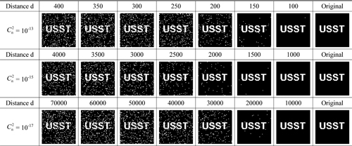
In the simulation, a 64 × 64-pixel binary image (letters “USST”, white on black) for correlation imaging has been selected, and the multiplicative gamma-gamma model of turbulence has been introduced. Three parameters―the transmission distance
In the simulation, we use the
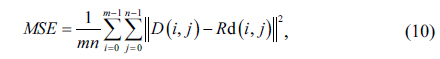
To detect the quality of the reconstructed image, two objective evaluation indicators, PSNR and BER, are used. Since the original image is a 64 × 64 binary image with only 4096 points, the image should be repeated to simulate enough points and calculate a sufficiently low BER. PSNR is an objective evaluation indicator for image quality, most commonly used in image processing. After compression, transmission, and other operations, the processed image usually differs from the original image. To measure the quality of the processed image, the PSNR value is usually used to determine whether the compressed transmission process conforms to the standard. PSNR is typically used for comparison of the maximum of the signal to the background noise. The larger the PSNR value between the two images, the less the distortion, and the more similar the two images are. PSNR can be calculated by Eqs. (10) and (11) as follows:

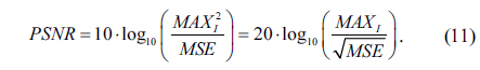
Here MSE is the mean square error between the original image and the output image, and
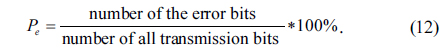
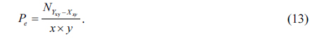
BER is also an indicator of the accuracy and reliability of a transmission system. It is defined as the ratio of the number of error bits to the number of all transmitted bits, as expressed in Eq. (12):

In this article, Eq. (12) is specified as:
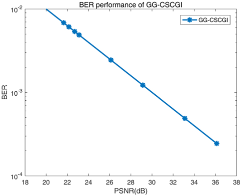
In Fig. 4, the relationship between the PSNR and the BER of a GG-CSCGI system is expressed. To eliminate the inherent error of the associated imaging,
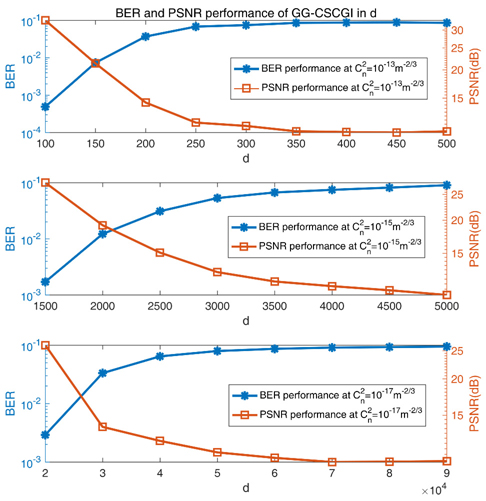
3.1. Analysis of the Influence under Different Conditions of Transmission Distance
To ensure that the associated imaging channel is only affected by turbulence,
[TABLE 1.] Imaging effects for different transmission distances (in meters)

Imaging effects for different transmission distances (in meters)
When and the value of
Obviously, as
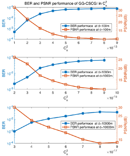
3.2. Analysis of the Influence under Different Conditions of Refractive-index Structure Parameter
Similarly, when analyzing the influence of ,
[TABLE 2.] Imaging effects for different values of the refractive-index structure parameter
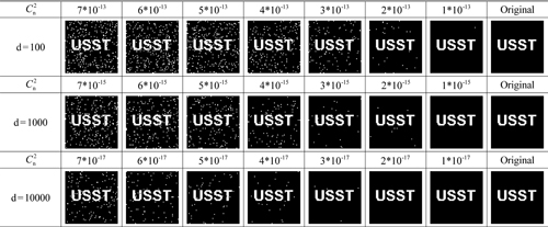
Imaging effects for different values of the refractive-index structure parameter
When
The trend in Fig. 6 is opposite than that in Fig. 5: As increases, PSNR rises, while BER declines. Both tend to stabilize when increases to a specific value that varies with
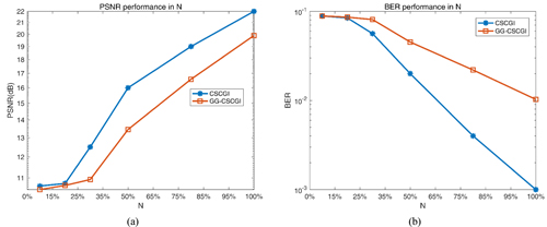
3.3. Analysis of the Influence under Different Conditions of Sampling Rates
Next the refractive-index structure parameter is taken as 1 × 10-15 and the distance
The corresponding image effects are shown in Table 3, and the PSNR and BER performance with varying
[TABLE 3.] Imaging effects under different sampling rates
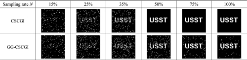
Imaging effects under different sampling rates
When
As
In this paper, the BER performance of a compressed-sensing computational ghost-imaging system based on the gamma-gamma atmospheric turbulence channel model has been researched. The influence of light intensity for the gamma-gamma atmospheric turbulence channel on image transmission has been analyzed. Specifically, the intensity influence is mediated by the key parameters of the turbulence channel, namely the refractive-index structure parameter and transmission distance