In recent years, the small UAV market has grown rapidly. Small UAVs are applied in various areas such as surveillance, reconnaissance, and aerial photography. In this small UAV market, many studies are underway especially for the Quadrotor. The Quad-rotor unmanned aerial vehicle is one that uses four rotors, which are equipped on the tips of crossshaped rods.
In addition, Quad-rotor aggressive maneuver researches are actively underway as well, with the aid of motion capture technology, which is a recent technology in this area [1-4]. In case of small UAVs, MEMS gyro sensors are used in many small UAVs, but MEMS gyro sensors have disadvantages that the error signal accumulates during the integration of measured data. However, position and attitude data can be measured with very high accuracy using the motion capture system, so that the system is capable of showing more precise control performance.
The GRASP laboratory of University of Pennsylvania has conducted aggressive maneuvers such as perching, or flips maneuvers. They used three different types of controllers for performing these maneuvers, and those controllers are categorized as an attitude control, a hover control, and a three-dimensional trajectory follow control. In other words, at one point, only one controller is used to control the Quadrotor system for each specific condition. When another condition for the Quad-rotor is met, then the controller switching logic is activated to switch the main controller to a different type of controller that is appropriate for the given condition [1].
In addition to this, the ACL at MIT has performed aggressive maneuvers with the variable pitch Quad-rotor [2].
This paper is composed as follows. First of all, the Quadrotor dynamic model is derived, and an appropriate control system is designed for the dynamic model of the Quadrotor. We use the conventional PD control method and sliding mode control method for the closed-loop control structure, and calculate input parameters for the open-loop control structure. To perform 6-DOF real time simulations, we assumed that the Quad-rotor flies in an indoor facility equipped with the motion capture system. Therefore we can also assume that measured position and attitude data of the Quad-rotor are very accurate.
2. Dynamic Modeling of the Quad-Rotor
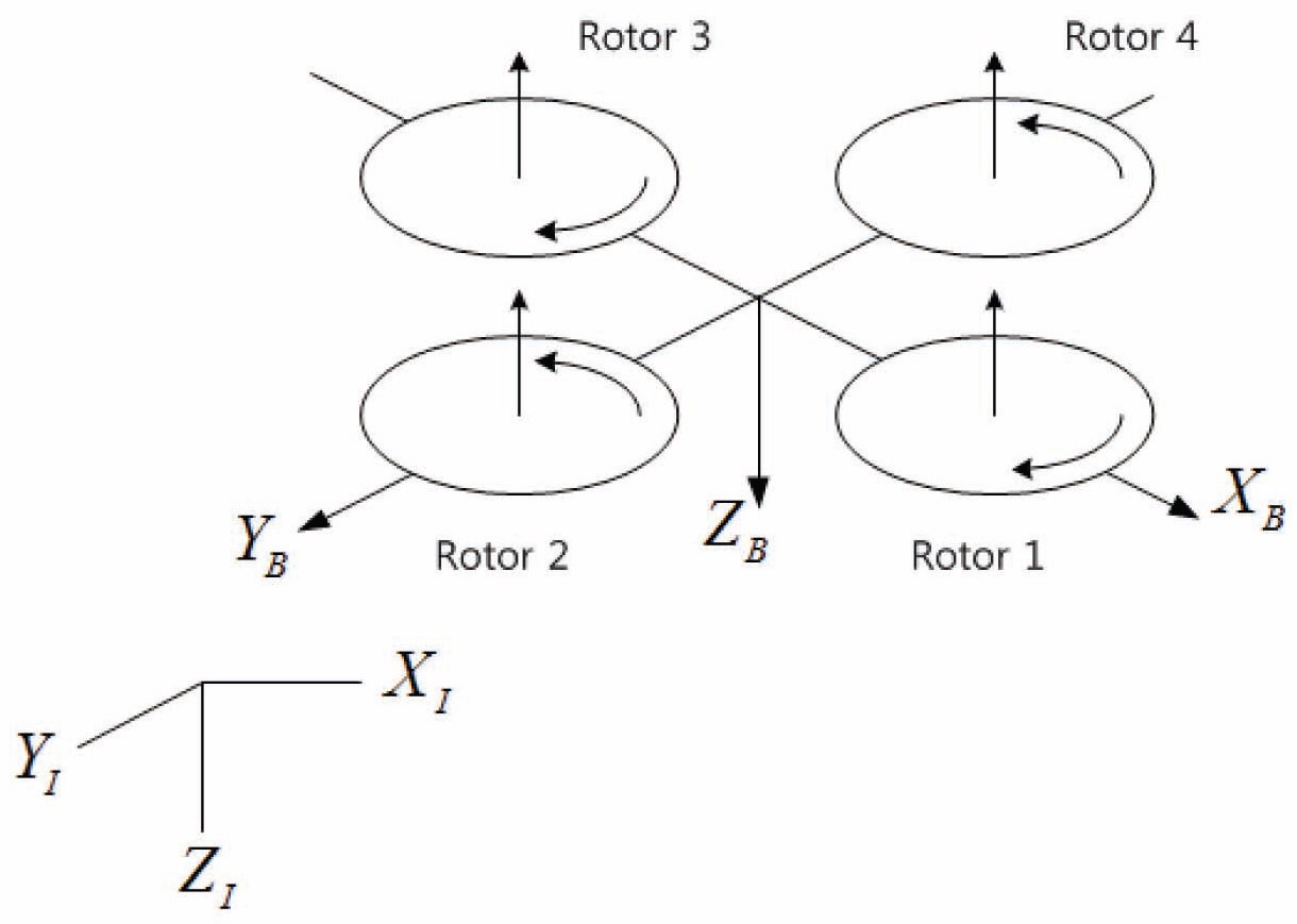
The Quad-rotor structure is shown in Fig. 1. This Quadrotor structure contains four rotors which are mounted on the tip of cross-shaped rods [5].
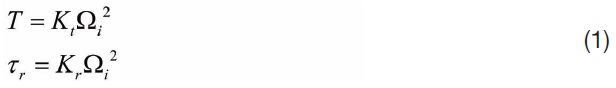
As we can see from Fig. 1, four rotors are defined as rotor number 1, 2, 3, and 4 in a clockwise direction from the front of the Quad-rotor. Quad-rotor Euler angles are changed by applying the angular velocity differences on these four rotors. We define the angular velocities ofrs as Ω1, Ω2, Ω3, and Ω4, and this actuator system is modeled as the first order system. The Equations (1) represent this actuator system.
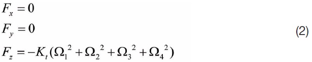
There are four rotors on the Quad-rotor, so forces acting in each direction of the Quad-rotor are expressed in Equations (2).
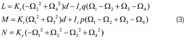
The moments acting on each angular direction of the Quad-rotor are shown in Equations (3), and these equations are considering the gyroscopic effect.
2.2 Quad-Rotor Control Allocation
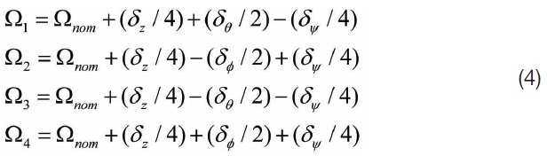
Typically, rotorcraft control commands can be determined as
3.1 Open Loop Attitude Control
Attitude control is for tracking and maintaining the Euler angles of the Quad-rotor. In this paper, three methods are used for designing the attitude controller. First of all, we use the open-loop control method for designing the attitude controller. To control the attitude of the Quad-rotor, one needs to generate system torques by controlling the angular velocity of each rotor, and the attitude rate of the Quad-rotor should be near zero when the Quad-rotor reaches the desired attitude. Since this method does not use any feedback control, this method is called the open-loop attitude control.
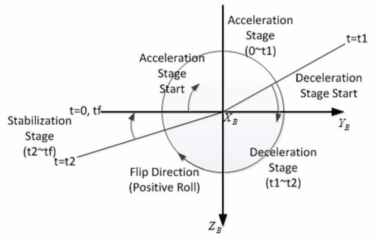
For this purpose, the system torque acting on the Quad-rotor is divided into three stages: acceleration stage, deceleration stage, and stabilization stage. During the acceleration stage, the Quad-rotor angular velocity should be accelerated to the maximum value. In contrast,
in the deceleration stage, the Quad-rotor angular velocity should be decelerated to the minimum value. Finally, in the stabilization stage, all rotors should rotate in the same angular velocities in order for the Quad-rotor to return safely to the original hovering state.
One good application is to consider the Quad-rotor performing a positive roll flip maneuver. We assume that the gyroscopic effect and disturbance are small enough to be negligible. A graphical representation for each stage of the flip maneuver is illustrated in Fig. 2. Before conducting the open-loop attitude control, the Quad-rotor should hold the hover state, then all rotors should rotate with the identical nominal angular velocity, Ω
In acceleration and deceleration stages, the torques and differences of angular velocities and Euler angles are as follows. In the acceleration stage, the angular velocity of rotor 2 decreases whereas the angular velocity of rotor 4 increases. Rotor 2 should rotate with the minimum angular velocity, Ωmin, and rotor 4 should rotate in the maximum angular velocity, Ωmax. Maximum and minimum angular velocities, Ωmax and Ωmin can be obtained as Equations (5).
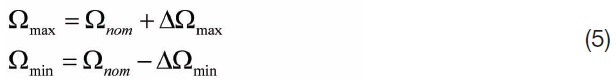
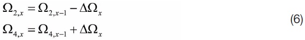
where ΔΩmax and ΔΩmin represent the changes in maximum and minimum angular velocity, respectively. In this paper, we assume that ΔΩmin = ΔΩmax, and it indicates that there is no extra torque generated from the flip maneuver except for the roll torque. In addition, the hovering stage, acceleration stage, deceleration stage, and stabilization stage are numbered as stages zero, one, two, and three, respectively. Now, in the
[Table 1.] Parameters of Open-loop control for each Stage
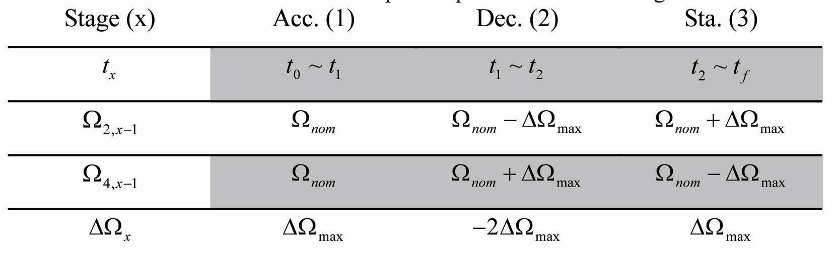
Parameters of Open-loop control for each Stage
Angular velocity variations in the
In this paper, the rotor system is modeled as a first order system with a time constant
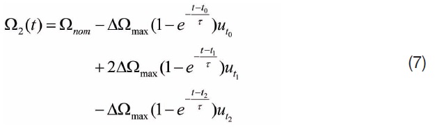
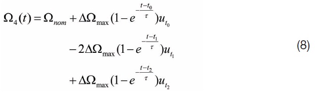
The angular velocity of rotor 4, Ω4(

Moment

Now, the moment sum during whole flip maneuver is defined as

We defined the Quad-rotor’s angular acceleration during the flip maneuver as
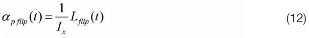
In addition, we can obtain angular velocities and Euler angles of the Quad-rotor at time t by integrating
[Table 2.] Quad-rotor Parameters
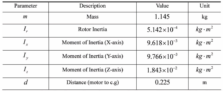
Quad-rotor Parameters
flip maneuver.
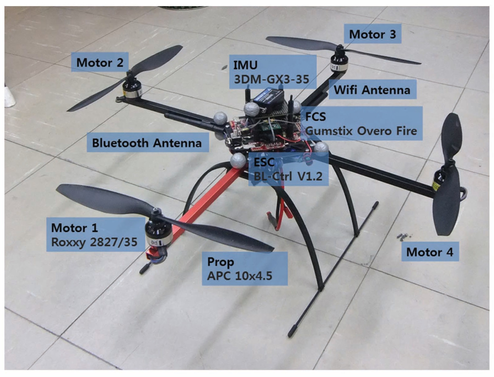
We built the Quad-rotor frame to determine parameters of the open-loop attitude control method. This frame is based on Mikrokopter Company’s Quad-rotor frame, and it is shown in Fig. 3.
Quad-rotor parameters are determined by measured data and calculated data using a previously built Quad-rotor frame as shown in Table 2.
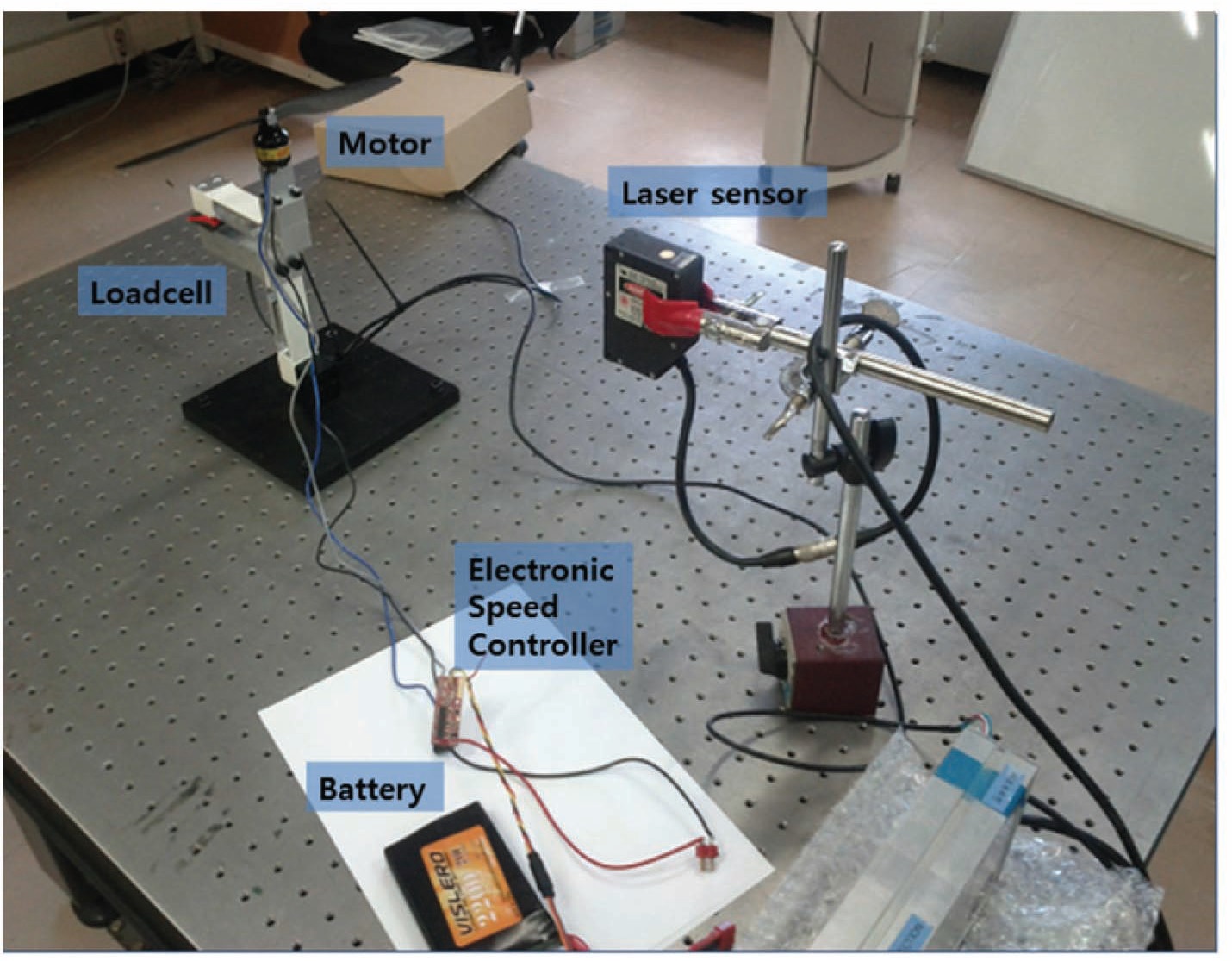
The thrust system of the Quad-rotor frame is composed of a propeller, motor, ESC and battery. The Thrust test was performed in order to measure the thrust coefficient and torque coefficient of the thrust system. The test environment has been set up as shown in Fig. 4. At this time, the rotor thrusts are measured by load cell, and the angular velocity of the rotor are measured by the laser sensor simultaneously.
By observing the thrust test results, the thrust coefficient is determined as
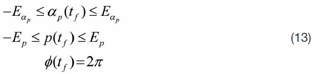
Now, we are going to calculate time
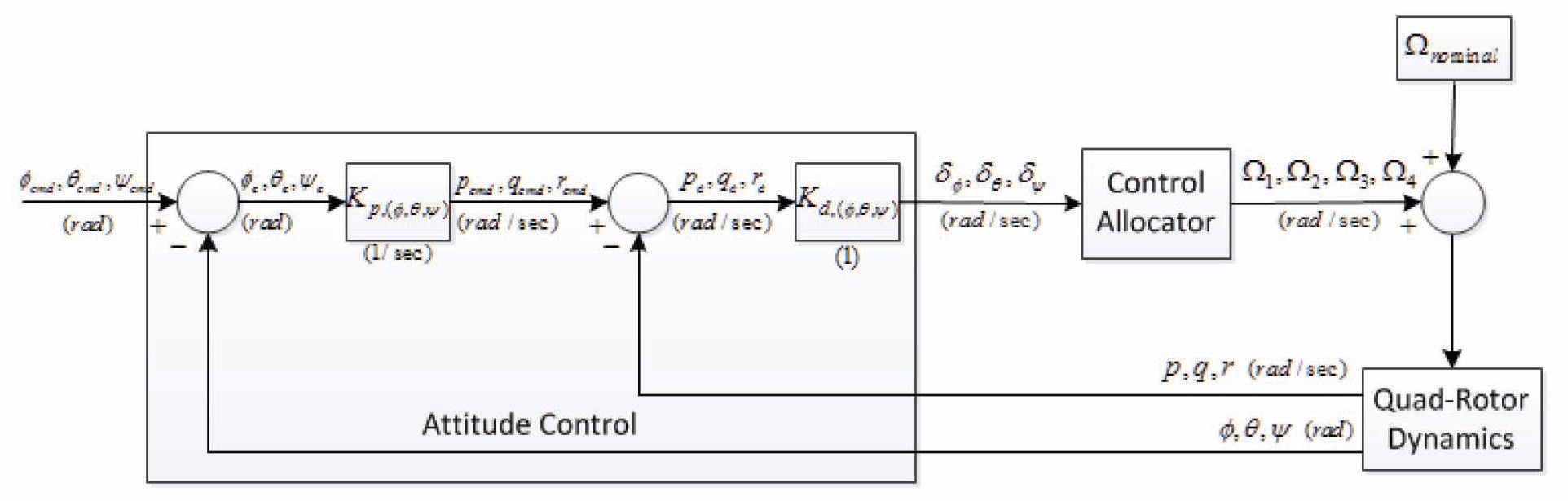
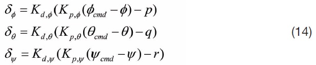
In this subsection, we use the PD control method for designing the attitude controller. Equations and structure of the PD attitude controller are shown in Equations (14) and Fig. 6.
[Table 3.] Parameters of Thrust Models
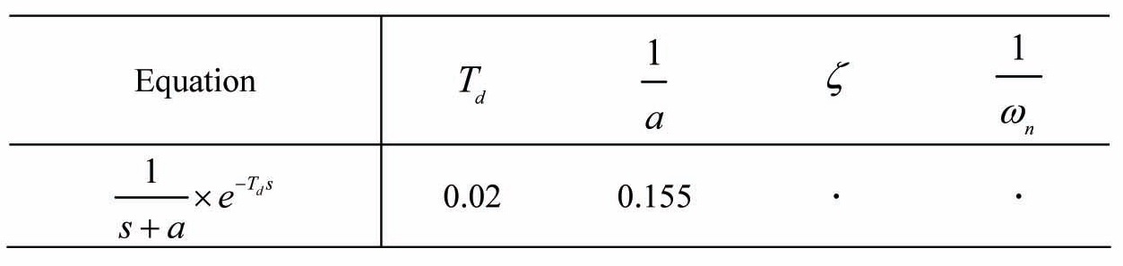
Parameters of Thrust Models
3.3 Sliding Mode Attitude Control
We can use the sliding mode control to conduct the Quad-rotor’s aggressive maneuvers. A brief introduction of the sliding model control is presented below [6-8]. Tracking error

is defined in Equation (15).

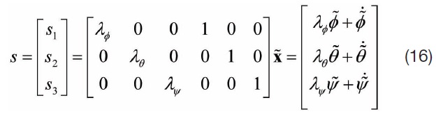
At this time, sliding surface s is defined by Equation (16).
If
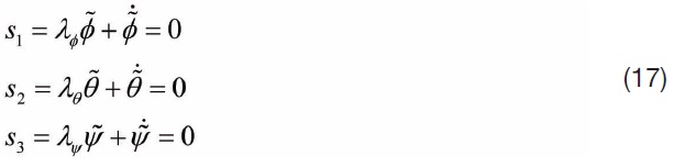
If
and

have the opposite sign, therefore we know that the sliding surface will converge to zero. Now, to make
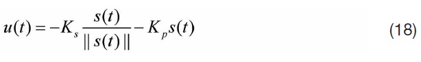
Here,
4.1 Attitude Control Simulation using Open Loop Attitude Control
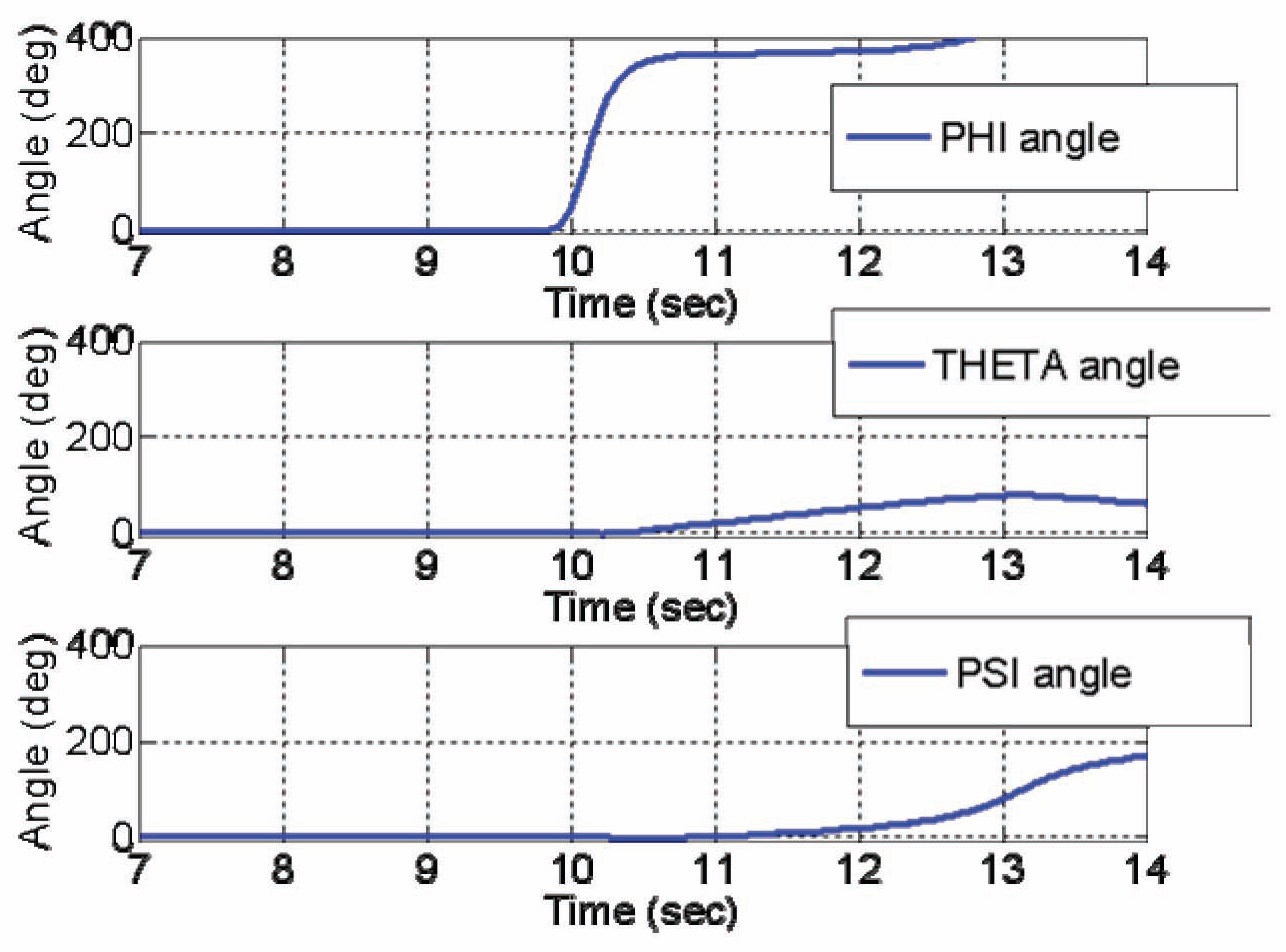
In this subsection, we perform the flip maneuver simulation using the open-loop control that we introduced in section 3.1. Parameters for the open-loop control are the
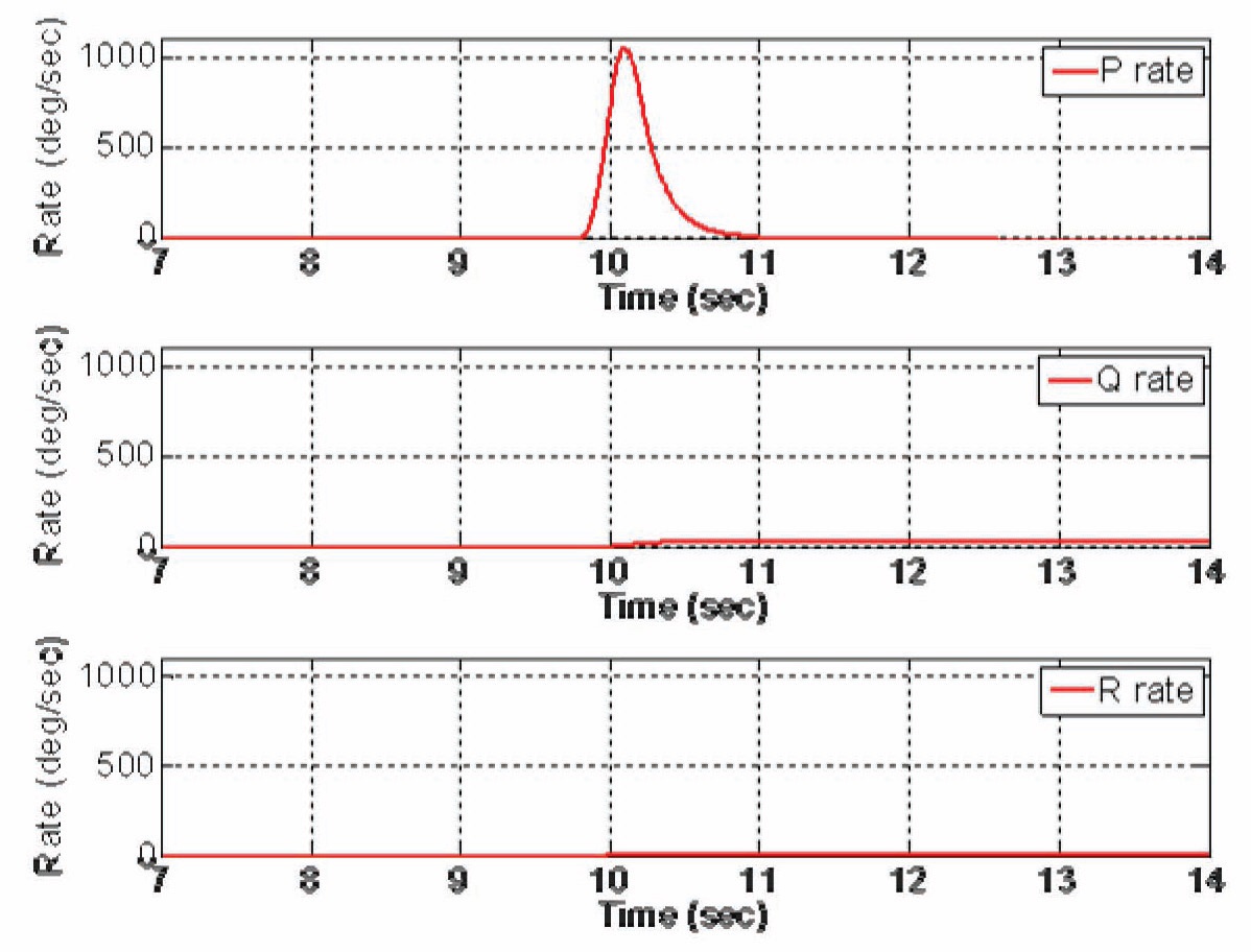
same as those introduced in section 3.1. Simulation results of the Euler angles are shown in Fig. 7, and Simulation results of angular velocities are shown in Fig. 8. As we can observe in Fig. 7, the Quad-rotor’s Euler angle
There are many reasons why the Euler angle
4.2 Attitude Control Simulation using PD Attitude Control
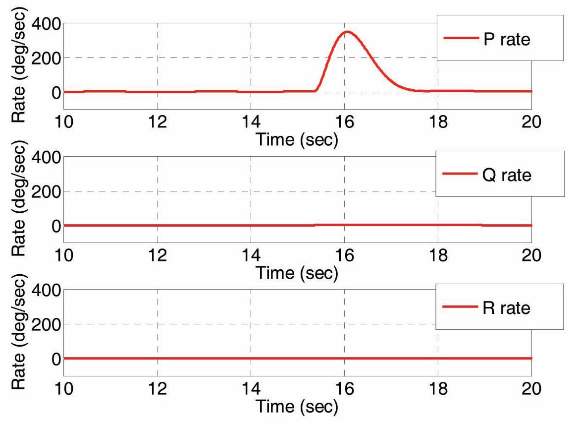
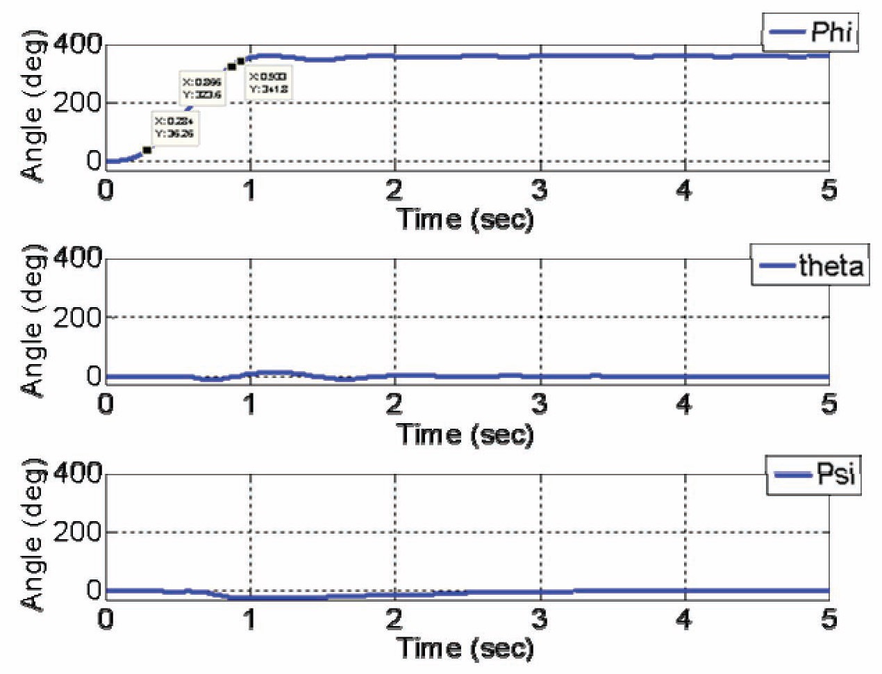
In this subsection, we use the PD attitude controller to simulate the flip maneuver. Simulation results of Euler angles are shown in Fig. 9, and simulation results of angular velocities are shown in Fig. 10. From the simulation results, the PD attitude controller takes about two seconds to accomplish the flip maneuver. We also know that maximum p is approximately 350 deg/sec. As we can observe from the simulation results graph, rise time is about 1.17 seconds and settling time is about 1.64 seconds. Comparing these results with the simulation results of the open-loop flip maneuver that we described in section 4.1, we find that the accomplish time for the flip maneuver of the PD attitude controller is remarkably slower than using the open-loop control results. However, simulation results of Fig. 5 do not consider the gyroscopic effect, so these results do not represent all simulation results of the open-loop control.
4.3 Attitude Control Simulation using Sliding Mode Attitude Control
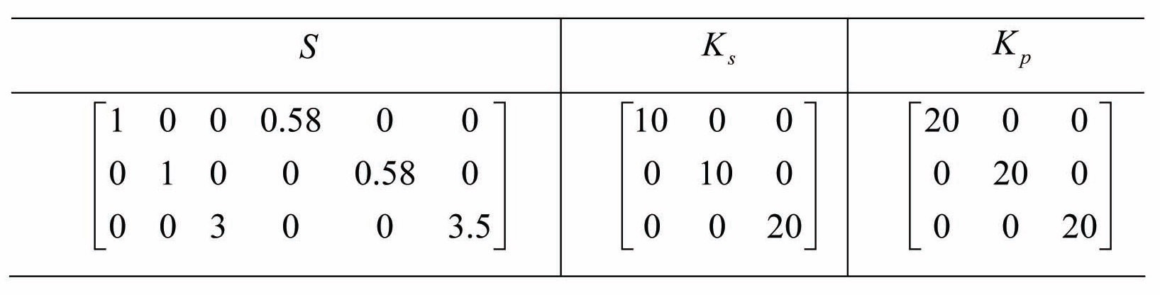
In this subsection, simulation results of the flip maneuver using sliding mode control will be presented. Parameters of sliding mode control such as
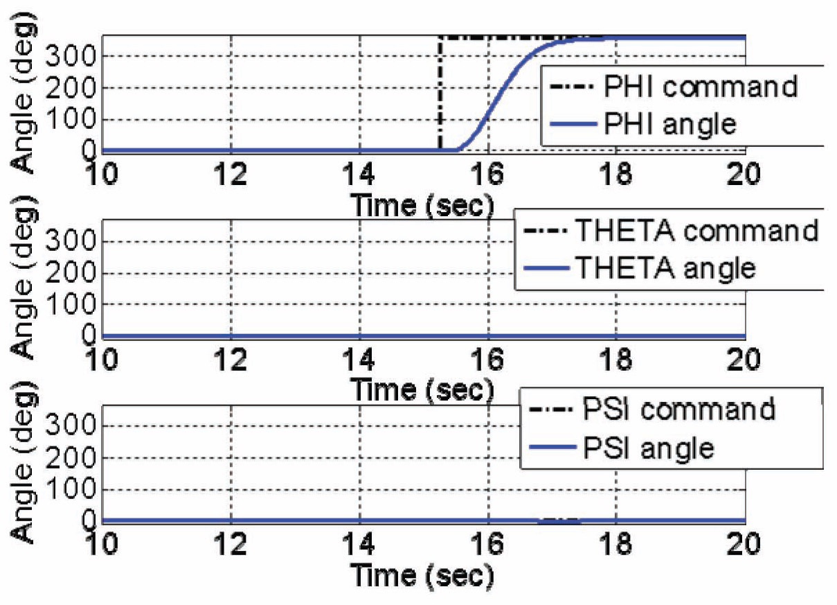
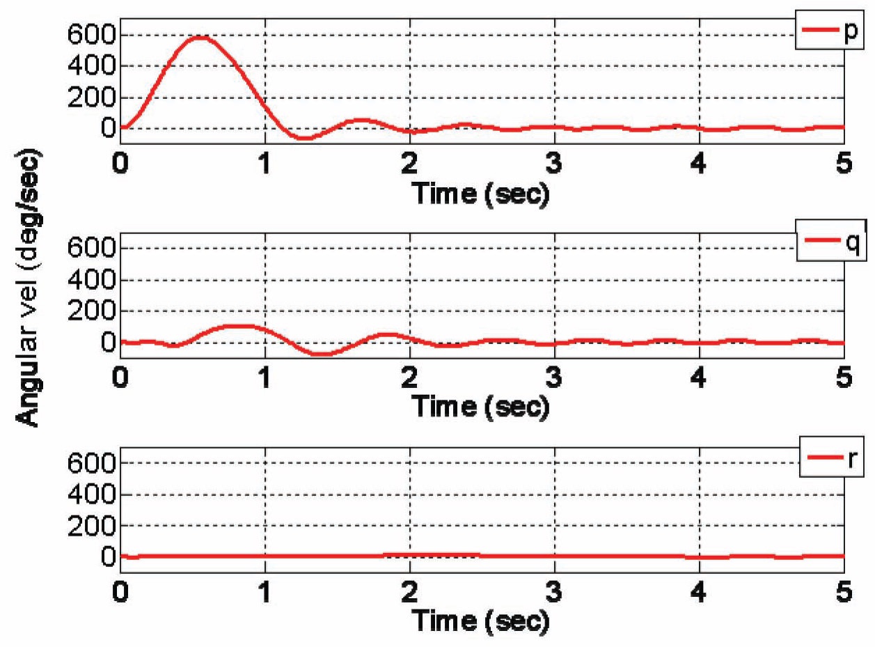
Simulation results of Euler angles are shown in Fig. 11. Simulation results of angular velocities are shown in Fig. 12.
As we can observe in Fig. 11, rise time of sliding mode control is approximately 0.58 seconds and settling time is about 0.93 seconds. Angular velocity
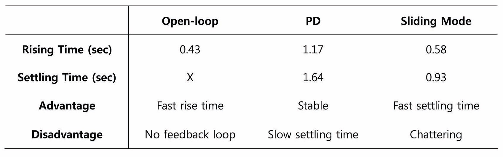
4.4 Performance Comparison of Attitude Controllers
Until now, we performed high angle control using three attitude controllers. Characteristics of these controllers are listed in Table 5.
In this paper, three attitude controllers of the Quadrotor were designed by various methodologies to perform a flip maneuver and we also compared performances of these attitude controllers. For this purpose, 6-DOF dynamic equations were derived and the Quad-rotor frame was configured. Here, we assumed that the aerodynamic components are small enough to be negligible. To control the attitude of the Quad-rotor, we designed three types of controllers. First, the open-loop controller was designed for the attitude control and the conventional PD controller was designed second. Lastly, the sliding mode control method was used to design the attitude control of the Quad-rotor. We simulated a flip maneuver using these three attitude controllers and compared performances of these attitude controllers. In case of the open-loop control
[Table 4.] Parameters of Sliding Mode Control (Simulation)

Parameters of Sliding Mode Control (Simulation)
[Table 5.] Performance Comparisons of Three Attitude Controllers

Performance Comparisons of Three Attitude Controllers
system, convergence speed is fast, but failed to hold the stability of the system. In contrast, the PD control system satisfies successful stabilization of the Quad-rotor with one drawback: convergence speed is slower than that of the open-loop control system. Finally, the sliding mode control system satisfies both convergence speed and stabilization. However, we can observe that there is chattering effect when sliding surface