Wind turbines operate in an aerodynamic environment which is difficult to analyze and predict. The periodic and aperiodic unsteadiness of the atmospheric boundary layer makes the design of wind-energy systems very difficult since their design is typically optimized for steady state conditions. In particular, the performance of the turbine blades is strongly affected by the stochastic nature of the airloads; the blade structure needs to be built for the best efficiency in converting the wind energy into usable mechanical energy while maintaining structural integrity [1-4]. The need to account for the random nature of the airloads leads to heavier, stiffer blade designs that are not optimized for the prevailing operating conditions. Also, the heavier blades limit the rotational speed of the rotor as the inertial forces acting at the root of the blades are too high for safe operation. The less-than-optimal design of the blades leads to higher initial and operating costs since centrifugal and gravity loads are primarily responsible for fatigue failure [1-4]. These design weaknesses are contributing factors to the competitive disadvantage of wind energy against other forms of renewable and non-renewable energy sources.
Options to improve the efficiency of wind turbine blades are varied. On one side of the spectrum there is the option to design lighter, stronger blades using more advanced materials. However, the high costs associated with the advanced structure and materials make this option economically not viable On the opposite side of the spectrum is the implementation of an active control system that, rather than modifying the blade structure to make it stronger and stiffer, allows the blade to morph and to change its shape in order to alleviate the instantaneous loads. By using this control strategy, the blade structural loads can be reduced and the operation of the wind-turbine can be continued under adverse environmental conditions. An additional advantage of an active control system is the effective stabilization of the blade which protects the wind turbine system against aeroelastic instabilities [5,6].
However, the proposed control system concept needs development and verification. In order to achieve these goals, an aeroelastic model that couples the blade structural response to the unsteady aerodynamic loads is being developed. In order to validate the control system as a proofof- concept, the aeroelastic model needs to be able to capture the characteristic behavior of both the fluids and structural domains and yet be relatively low-cost for quick turnaround design iterations.
One of the bottlenecks in the development of the aeroelastic model is how to best capture the aerodynamic behavior of the blade since such a prediction is critical to the reliable description of the system. Often aerodynamic modeling has been accomplished by means of engineeringtype empirical models like the ONERA or the Beddoes- Leishman models [7,8]. The airloads models are based on the conventional rotorcraft lifting line approach of treating each 3D rotor blade as a series of 2D airfoil sections and calculating the section airloads based on local section aerodynamic parameters. This is mainly due to the fact that the considered blades have large aspect ratio. In addition, the aerodynamic loads are based on the blade element momentum theory which assumes a 2D flow over each blade airfoil section. The induced velocity is obtained from the simple momentum theory, generalized dynamic wake, prescribed wake, or free wake. Static stall and compressibility effects are implicitly included in tabulated data as functions of angle-of-attack. Another assumption is that the quasi-steady aerodynamics governs the reverse flow region. Navier-Stokes solvers have been usually restricted to two-dimensional analysis and only a few attempts have been made to advance the state-of-theart in aeroelasticity from two-dimensional to quasi-threedimensional and fully three-dimensional Navier-Stokes solutions [9,10].
In this paper, the aerodynamic loads are computed using Computational Fluid Dynamics (CFD) techniques. A commercial finite-volume code, FLUENT®, that solves the Navier-Stokes and Reynolds-Averaged Navier-Stokes (RANS) equations is used. Turbulence effects, considered only in the 2D simulations, are modeled using Wilcox’s
Desired outputs from this numerical tool are the vibration levels due to the unsteady loads acting on the rotating wind-turbine blades, and the prediction of the fatigue-life of the structure and the exterior noise of the operating wind turbines. Ultimately this effort is meant to provide the wind turbine industry with a tool for the design of more efficient wind turbines.
2. Computational Fluid Dynamics Model
The CFD model of the blade was developed using a commercial CFD code, Fluent 6.2 [14]. Fluent was chosen due to its validated performance and availability of physical models and widespread presence in the power generation industry. The blade geometry was reconstructed in the mesh generator, Gambit 2.3, from the data provided in Giguere and Selig [17]. The 3D simulations were run using the fully 3D unsteady laminar Navier-Stokes (NS) equations. Note that while the flow is turbulent, unsteady laminar simulations were used in consideration of the fact that the present work presents a methodology and develops a tool for the aeroelastic analysis of slender wind turbine blades which is independent of the unsteady nature of the flowfield. That is, the same methodology and workflow philosophy that can be applied to a laminar flow can also be used for a turbulent flow, and this flexibility is part of the appeal of the present method. The intent here is to provide the reader with a recipe on the procedure to follow in wind turbine rotor fluid-structure simulations, which has a general value, independently of the qualitative nature of the CFD simulations. In future work the extension to a turbulent fluid model will be presented. The 2D simulations were run using the unsteady Reynolds- Averaged Navier-Stokes (URANS) equations and turbulence effects were computed using the Wilcox
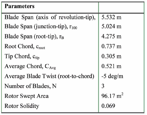
[Table 1.] Blade and Rotor dimensions

Blade and Rotor dimensions
incompressible and a pressure-based solver was employed. Second-order upwind spatial discretization was used for the transport equation and a second-order Runge-Kutta scheme was used for time discretization [14].
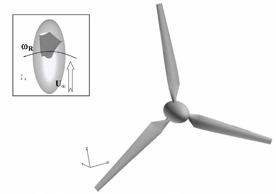
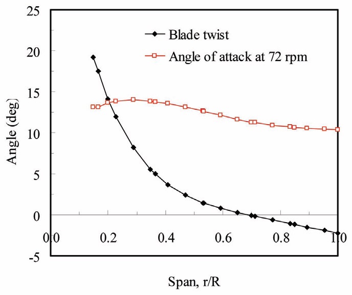
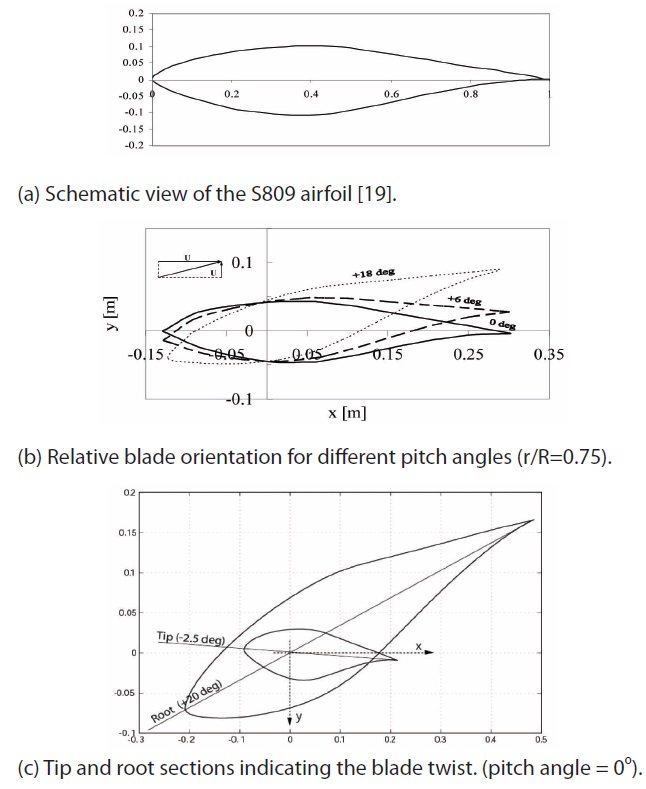
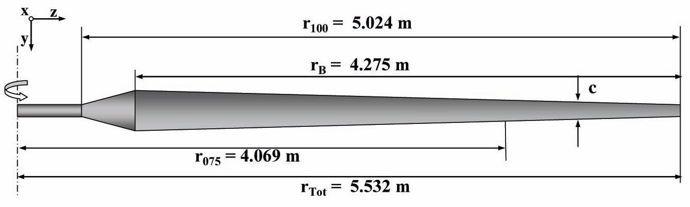
The geometry of the wind turbine and the definition of the boundary conditions with a uniform velocity inlet profile, allows the use of rotationally periodic boundary conditions so that only one single blade has been simulated. The blade geometry is shown schematically in Fig. 1 and the blade dimensions are summarized in Table 1. The blade twist is plotted together with the nominal angle-of-attack for a rotational speed of 72 rpm in Fig. 2.
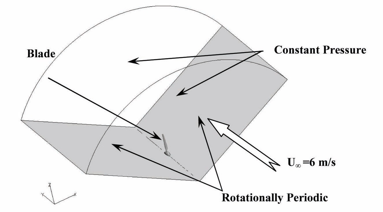
Additional geometrical parameters are provided in the numerical results, Section 4. The computational domain, shown in Fig. 3, comprises a section of a cylinder 120° in arc. The radial dimension is 30 m and the domain extends 15 m in front and aft of the rotor so as to minimize any influence from the boundary conditions. The operating conditions for the simulations are summarized in Table 2. A uniform steady velocity profile of 6.0 m/s was used for the upstream boundary condition while a constant-pressure boundary condition was used for the downstream boundary condition
[Table 2.] Summary of the flow conditions, ISA sea-level
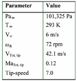
Summary of the flow conditions, ISA sea-level
and for the side at the plane of maximum radius. An axis boundary condition was used for the axis of rotation of the rotor and rotationally-periodic boundary conditions were applied at the two side planes.
The computational mesh is a hybrid mesh that contains both hexahedral and tetrahedral elements for a total of 1.14M cells. The hexahedral elements are primarily used to construct a finer mesh on the solid surfaces of the turbine so as to capture the viscous effects of the boundary layer. A canonical grid convergence study was not performed for the present work although solution-steered grid adaption was performed to study the sensitivity of the force and momentum results to mesh refinement which was found to be minor for the present conditions.
2.3 2D/3D Aerodynamic coupling
In this work 2D and a 3D aerodynamic models have been compared. The 2D model enables one to calculate the inflow ratio, denoted as

through a combined blade-element and momentum theory. It is possible to write [15,23]

where
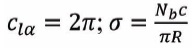
(see Table 1);
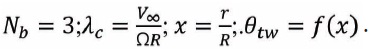
In the previous equation,
is a function of the local spanwise distance

could be estimated from the knowledge of the effective angle of attack gained from the 3D CFD. The sequence to evaluate the inflow ratio for the 3D case is as follows:


First, the effective angle of attack,

is evaluated from Eq. (2b). At this point, the values of

and
are different, therefore, Eqs. (2a) and (2b) are iteratively solved until Eq. (2c) is satisfied. Note that ε is a small arbitrary quantity and for the present simulations it was set to 1x10⁻⁵. The coefficients
Assuming the structural behavior of the windmill blade equivalent to a rotating beam, the corresponding mathematical model has been derived from the nonlinear flap-lag-torsion equations of motion presented in Hodges et al. [11]. In this representation, the blade is a cantilever, straight, slender, homogeneous, isotropic with nonuniform properties, with twist and both mass and tensile offsets. The resulting equilibrium equations are further simplified neglecting those terms considered to be of the third order with respect to the bending slope, that is an arbitrary small parameter, and not contributing to damping. Moreover, in this set of equations the radial displacement is not explicitly considered since the corresponding local tension is used. Therefore, the bending deflections are not responsible for the windmill blade axial extensions that are simply geometrical consequences of the transverse bending deflections [19]. Taking into account the previous assumptions, the dynamic system is represented by a set of coupled nonlinear integro-partial differential equations suitable for describing significant deflections [19,20] of the windmill blades where the unknown state is represented by the in-plane displacement of the elastic axis,
The aerodynamic load, used to couple the previous equations of motion, is based on the low-frequency approximation of two-dimensional Greenberg theory [12], leading to a simple quasi-steady strip-theory capable to take into account a pulsating free-stream for an unsteady aerodynamic loads acting on a thin airfoil. In this formulation, a first coupling with the 3D aerodynamic calculations is introduced. The local section aerodynamic parameters are evaluated from the results of the CFD calculations described in the previous section. Moreover, the aeroelastic model is completed by including the effects of the flow induced by the wake on the blade angle-of-attack as resulting from Eqs. (2a)- (2c). Again, considering the aerodynamic 3D calculations as an experimental test bed, the changes of the angle-of-attack due to the induced velocity could be estimated from the velocity changes of the flow through the actuator disk, as reported in the previous section and in [12] and [13].
The resulting final aeroelastic system could be integrated in the space domain using the Galerkin approach adopting the non-rotating modes of the blade as shape functions. If

are the linear time-invariant mass, damping and stiffness structural and aerodynamic contributions, and

represents the set of all nonlinear and/or time-dependent coefficient terms, then the set of the nonlinear ordinary differential equation is written as

where
The dynamic hub loads (root shears and moments) corresponding to the aeroelastic deformation, achieved from the previous solution, could be evaluated in the rotating frame. Then, the hub loads in the fixed frame of reference could be achieved by adding the contributions from all the blades expressed in the inertial frame of reference. If the drag, radial, and vertical shear forces at the rotor hub are denoted as


In this section, the results from both the aerodynamic and aeroelastic simulations are reported. In the following subsection, after a general description of the wind turbine model used in the numerical analysis, the results from the aerodynamic simulation of the rotating S809 airfoil are first outlined, then the results from to the aeroelastic simulations are presented.
4.1 Main characteristics of the NREL S809 wind turbine
The work focuses on a small wind-turbine blade designed to operate on a stall-regulated downwind wind turbine having a rated power of 20 kilowatt.
The blade geometry and dimensions were extracted from the National Renewable Energy Laboratory (NREL) experiment setup [17,18,21,22], and some of these parameters are reported for completeness in Table 1. The rotor diameter is 11.06 m with a root extension from the center of rotation to the airfoil transition of 0.88m, see Fig. 4. The blade is twisted (root twist of 20°, tip twist of -2.5° about the 30% chord location) and tapered (root chord of 0.737 m, tip chord of 0.305 m) and it features a NREL S809 airfoil with a thickness ratio of 21% (see Figs. 4 and 5) [21]. The blade pitch ratio is referenced to the 75% span location, see Fig. 4, and it is defined with respect to the x- and y axes, as shown in Fig. 5(c). The three-bladed rotor has a solidity of 0.069 and it rotates at 72 rpm with a uniform inflow speed of 6 m/s, giving a tip-speed-ratio of 7.0. An ellipsoid of revolution is located between the blade root extension and the axis of revolution of the rotor to maintain a smooth and realistic flow field
around the root region.
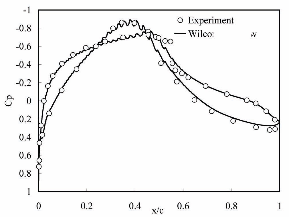
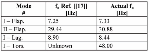
This section presents the results of the aerodynamic modeling of the rotor. First, a validation study of an S809 airfoil was performed to demonstrate the validity of the CFD approach to calculate the loads on the blade structure. In Fig. 6 the pressure coefficient distribution along the chord of the wind turbine blade is presented achieved with the reference flow conditions reported in Table 2.
The predicted Cp distribution is in overall excellent agreement with the experimental data with the exception of the location at 55%c where a mild flow separation is present and the CFD solution fails to predict its strength. The numerical solution shows noticeable oscillations in the Cp distribution in the region ahead of 55%c. The oscillations are indicative of an incipient flow separation on the upper surface of the airfoil. Comparisons for the drag, lift and
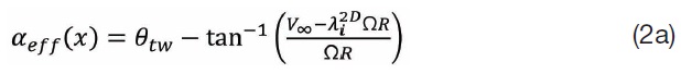
[Table 3.] Comparison of moments and forces for the 2D calculations.
Comparison of moments and forces for the 2D calculations.
moment coefficient of the present work to experimental results [21] and the Wolfe and Ochs CFD simulations [22], where the
The comparison shows some discrepancy between FLUENT® results and the experiments reported in Somers [21], especially for the drag coefficient which is 37% larger than the measured value. One source of error is the lack of detailed information on the inlet boundary conditions used in the experiment. In the present CFD simulations a uniform inlet velocity profile with a freestream velocity of 48.5 m/s was used to match the experimental Reynolds number of 2.0x10⁶. Additional source of error is the use of a viscous laminar flow model even at high Reynolds number where turbulence flow might significant effect, with potential effect also from turbulence boundary layer and trailing edge separation. These are all issues of great importance when looking into accuracy of the fluid-flow numerical simulations. Inlet turbulence was set at a turbulence intensity, TI=k/(u∞)2 , of 5% and at a turbulent viscosity ratio,
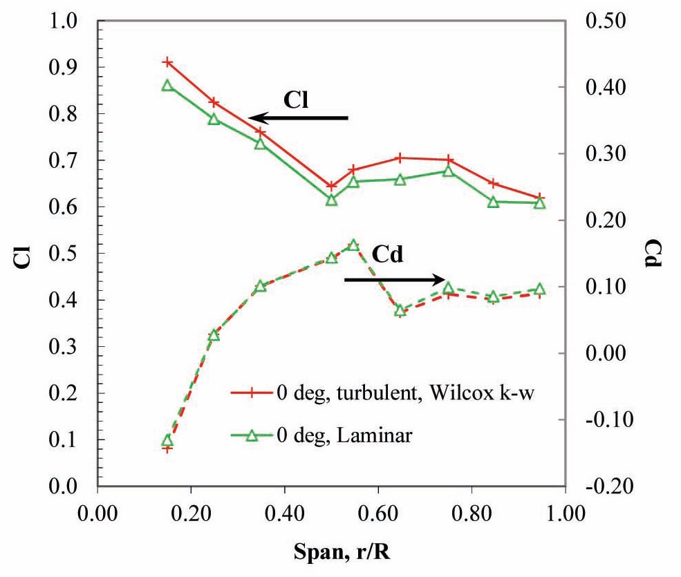
three-dimensional blade for a nominal angle of attack of 0 deg. The results are presented in Fig 6a.
While the absolute forces produced by the laminar and turbulent simulations are different, as expected, there is an overall similarity in the results, especially for the Cd. Also, it is important to notice that the methodology here proposed is valid for both flow regimes. Therefore, the 3D simulations were run without turbulence modeling. Also, laminar conditions might exist in some specific situations but in general it will be up to the designer to check the flow regime and run the appropriate flow model.
It is worth mentioning that other realistic computational techniques, such as the strip-theory, could be adopted in conjunction with 2D turbulence computations. As an example, the performance of several 2D turbulence computations at a number of axial positions along the blade could be performed and the formulation of an approximate 3D loading for the full length of the blade would then be a feasible option. This was however well beyond the scope of the present paper and it is left to the interested reader to pursue this or other viable approaches.
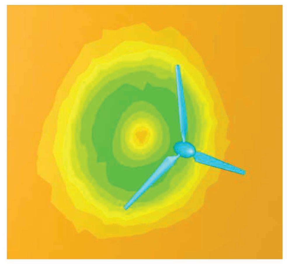
Figure 8 shows the momentum deficit of the incoming flow once it has passed the rotor. In this isometric view the rotor is shown in full and the hub is included for clarity. The relative high-momentum in the undisturbed region away from the rotor and in the small region of undisturbed flow near the axis of rotation is clearly noticeable. The latter highlights the action of the turbine blades that are extracting linear momentum from the incoming air flow to turn it into rotor rotational momentum. The use of rotationally-periodic boundary conditions in the 3D simulations allowed the study of the blade-wake interaction. However, from monitoring the force time history, it appears that for a rotor angular speed of 72 rpm and an undisturbed airspeed of 6 m/s (tip speed ratio of 7.0) the interaction is almost negligible.
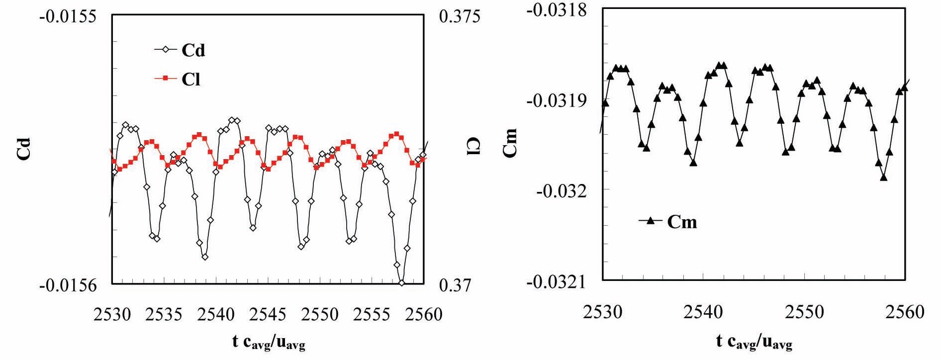
The time history of the lift, drag and moment coefficient on the blade, Fig. 9, show a Strouhal number based on a blade average chord of 0.521 m and an average blade velocity of 26.7 m/s of 0.22, corresponding to a dimensional shedding period of 0.09 s, also confirmed by a Fast Fourier Transform analysis of the force data. This period is shorter than that of the wake shed by the preceding blades, 0.278 s
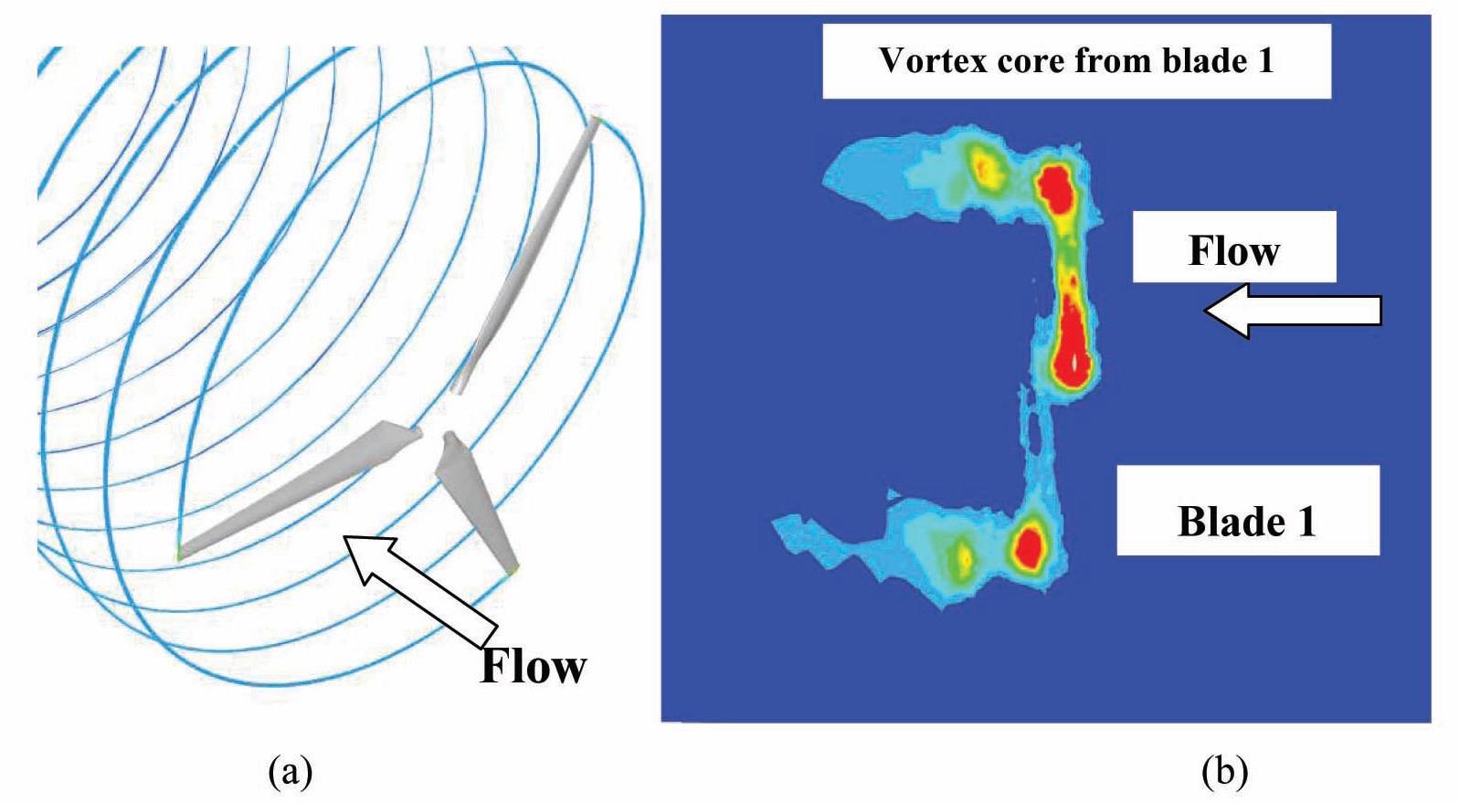
and it is attributable to the natural shedding frequency of the blade. Notice also that the amplitude of this oscillation is relatively small, 0.27% of the mean value for the drag and moment coefficient and 0.16% of the mean value for the lift coefficient. The blade-wake interaction is also visualized in Fig. 7(a) where the streamlines originating from the blade tips are plotted as they are convected downstream. The picture shows that the blades are well clear of the wake core produced by the preceding blade. Fig. 7(b) maps the vorticity contours on a flat plane normal to the blade axis at r/R = 0.75. The mapping shows the vortex chores from the main blade whose cross section is visible at the center of the map. The vortex chore coming from this blade, blade 1, is visible traveling downstream in the upper center of the figure. The vortex chore produced by the preceding blade is also visible before and after it approaches the azimuthal location of blade 1. Again, the mapping highlights the weak interaction of the blades with the wake.
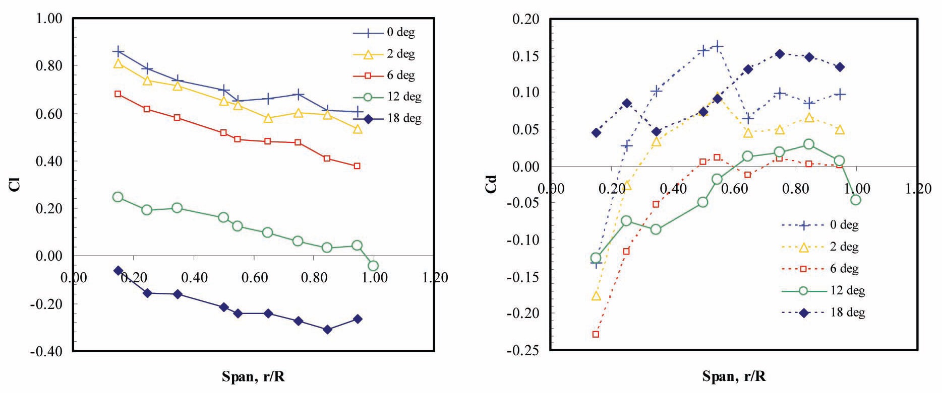
The lift, and drag coefficients for the blade at different pitch angles are plotted in Fig. 10 as a function of the blade span. The coefficients are computed using the dynamic pressure at the specific blade section and the angle formed by the local velocity vector. The plot of the lift coefficient shows a consistent trend at all pitch angles of decreasing
lift with span location. Also, the lift tends to decrease as the pitch angle is increased. The drag coefficient curves indicate two distinct trends depending on the pitch angle. At lower pitch angles, the drag increases steadily up to 50% of the span where it abruptly decreases, possibly indicating separation. This discontinuity decreases in intensity with increasing pitch angle and it disappears completely for a pitch angle of 12° and 18°.
Note that, at this location for the low pitch angles there is a minor drop in lift coefficient. According to the orientation of the axes or reference, a negative drag coefficient corresponds to a “forward” thrust for the rotor, the highest power is obtained for a blade pitch angle of 6 . Lower pitch angle settings are not producing as much thrust since most of the aerodynamic force is transformed in lift which is not contributing in a major way to the production of usable power. Also note that the overall thrust is given by a combination of lift and drag. Figure 11 shows the lift-curve of the different blade sections as a function of angle-of-attack. The lift curve slope is 3.00 per radiant (0.95
The lower value of the 3D solution is due to the threedimensional effects of the blade. These effects were calculated following Bramwell [23] where the induced velocity,

Where
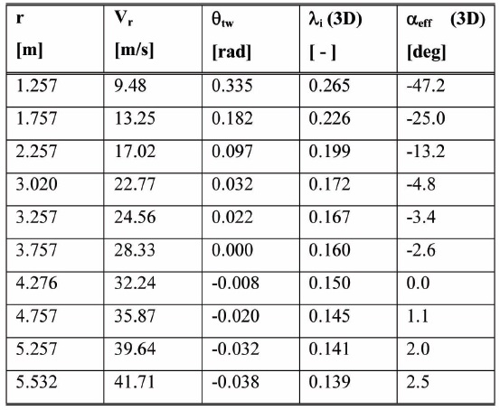
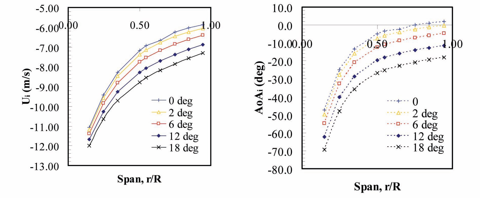
of blades of the rotor. The calculated induced velocity is shown in Fig. 12 together with the induced angle-of-attack. As expected the induced velocity is higher closer to the hub where the blade loading is generally higher. Also, the induced velocity is higher for the case with higher pitch angle and tends to decrease as the pitch angle is lowered.
The coefficients
[Table 4.] Fluent data for 3D model

Fluent data for 3D model
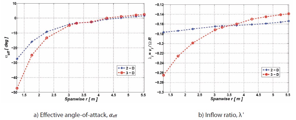
from the previous analysis are shown in Fig. 13; from these figures the different trend that occur for both
4.3 Structural blade characterization
As stated in the previous section, the nonrotating modes of the blade are required in order to solve the aeroelastic system
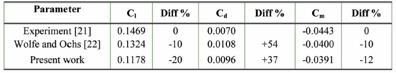
[Table 5.] Comparison between the reference and the actual modal model
Comparison between the reference and the actual modal model
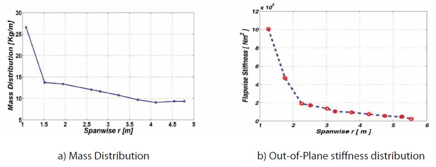
of equations. The flapwise and lag stiffness together with the mass distributions, required for setting up the modal model, have been evaluated using both the data reported in Giguere and Selig [17], and estimated from similar blades by using an approach based on the dynamic similitude. In Fig.14 the mass and the flapwise stiffness distribution as function of the blade span are reported, while, since no torsional stiffness data were available from [17], a typical value for this kind of blade, considered constant over the blade span, has been assumed. These structural characterizations lead to natural frequencies reported in Table 5. As one can see, the considered modal model is almost the same as the one identified in [17].
In Fig. 14 the mass and the flapwise stiffness distribution as function of the blade span are reported, while, since no torsional stiffness data were available from [17], a typical value for this kind of blade, considered constant over the blade span, has been assumed. These structural characterizations lead to natural frequencies reported in Table 5. As one can see, the considered modal model is almost the same as the one identified in [17].
4.4 Static Aeroelastic Simulation
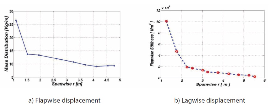
The aeroelastic simulation has been performed considering the windmill rotating at fixed operational conditions in terms of rotational speed and blade aerodynamic incidence. This condition is equivalent to consider the windmill operating at constant, ideal, wind flow regime. The solution of the system of aeroelastic equations is carried out through harmonic balance leading to the evaluation of the elastic deformation of the hingeless blade. Herein, the aerodynamic coefficients and the inflow distributions along the blade span due to induced velocity from the 3D calculations are taken into account. The static component of the flap and torsional deflections, for the blade azimuthal position ψ=0, are presented in Figs. 15 and 16.
It is noteworthy to observe that the flap deflection occurs in the wind direction (Fig. 15a), whereas the lag occurs in the direction of the rotational velocity (Fig. 15b). By comparing these results with the ones of a rotorcraft in hover with ascension velocity equal and opposite to the one of the wind
mill it can be noticed that the flap and lag are the opposite in directions; these results are consistent to the fact that a torque is produced at the hub of the wind mill by the interaction wind-blade system, while in the helicopter a torque at the shaft is provided by the propulsion system to generate the thrust. It is also clearly evident from these figures that the 2D model does predict lower flapwise deflections that the 3D model counterparts which is associated with the slightly increased effective angle of attack that is present in the 3D case, see Fig. 13a. On the other hand, the corresponding lagwise deflection is slightly lower, which might be associated with an over-estimate on the 2D aerodynamic loading. The different is quite small also considering also
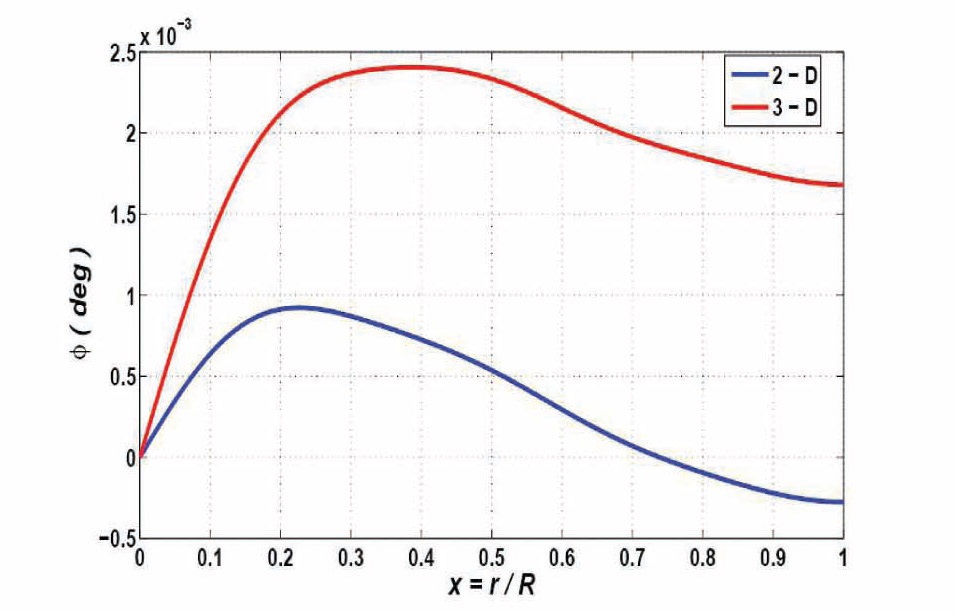
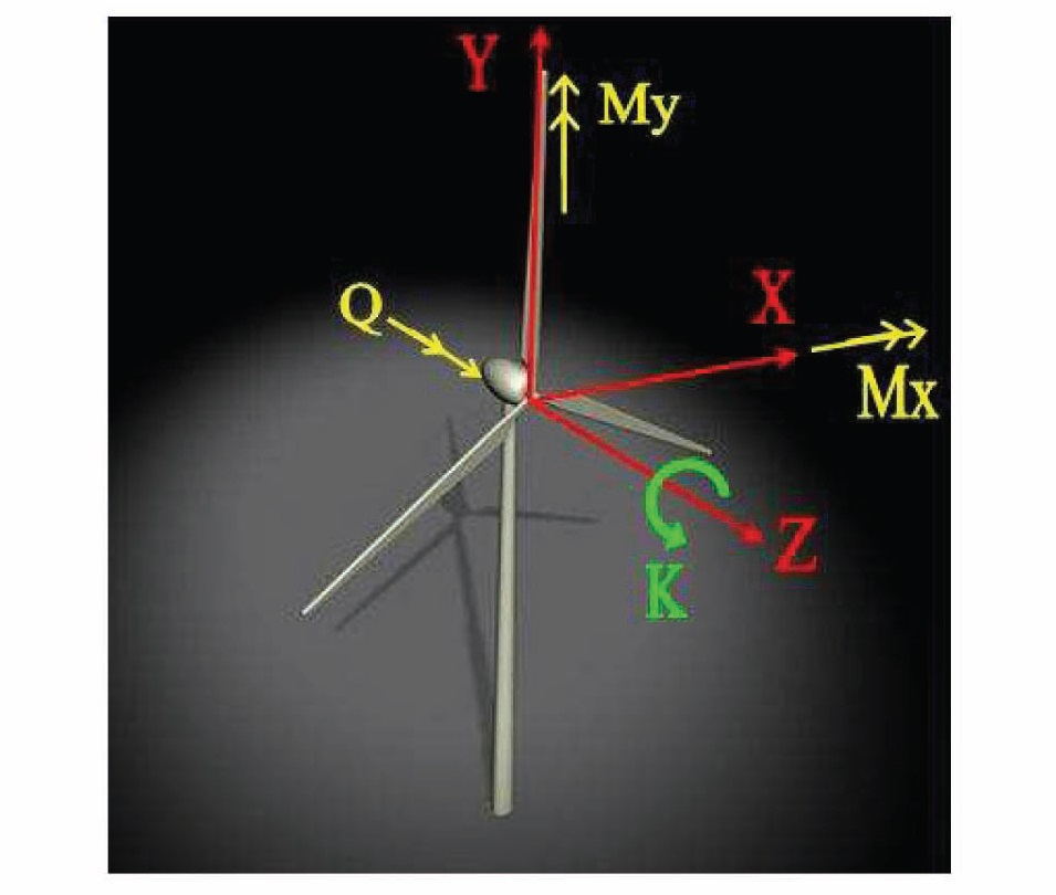
that in this direction the loads are one order of magnitude smaller and in the flapwise direction. The combined effect of flap and lag deflection contributes to a large discrepancy in the torsional direction, as it is displayed in Fig. 16. Clearly the inherent flexibility of the rotor combined with the complex aerodynamic characteristics in the spanwise direction creates some complexities in the deformation field and it is quite challenging to fully interpret. It is also possible to estimate the shear and moments along the span of the blade in the undeformed rotating reference frame attached to the blade, as reported in Fig. 17.
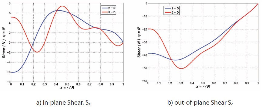
The comparison between the dynamic loads as function of the blade span, considered at ψ=0, are reported in Figs. 18 and 19 where the different evaluations of the dynamic
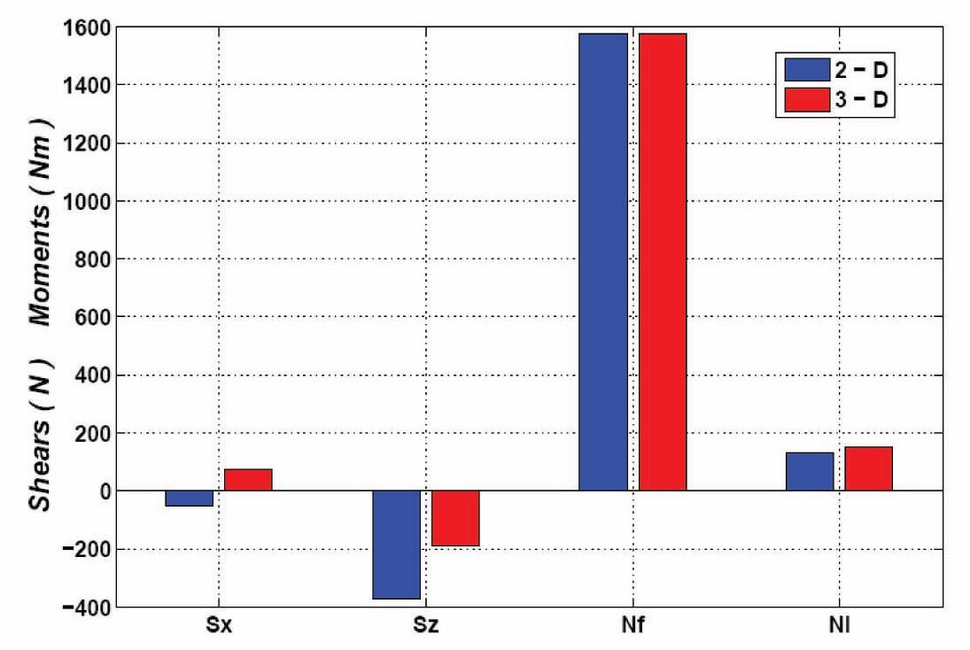
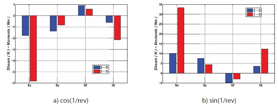
rotating shears and moments, are depicted. Moreover, the different hub load estimates, always in the rotating reference frame, are reported in Figs. 20 through 22. From Fig. 20, only a remarkable difference in the static out-of-plane shear is reported, whereas a completely different behavior, but with much smaller amplitudes, of the dynamic elastic reactions (acting at 3/rev and 5/rev harmonics), is evident in Figs. 21 and 22, respectively.
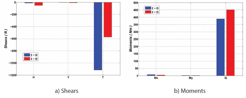
When considering the resulting loads acting in the fixed reference frame, the convention reported in Fig. 17 are used. For the positive values of the hub dynamic loads: the thrust, T, is developed by the rotor acting in the orientation of the wind; the torque, Q, (responsible for the power generation of the wind turbine) has the orientation of Ω; H and Y are the shears acting in the x and y reference directions, respectively; and, finally, Mx and My are the bending moments in the x and y axis, respectively. The aeroelastic loads evaluated in the fixed reference frame excite the windmill structure at discrete frequencies that are the number of blades of the rotor times the rotating angular frequency (see e.g. [20] through [22], [27]) plus the static component.
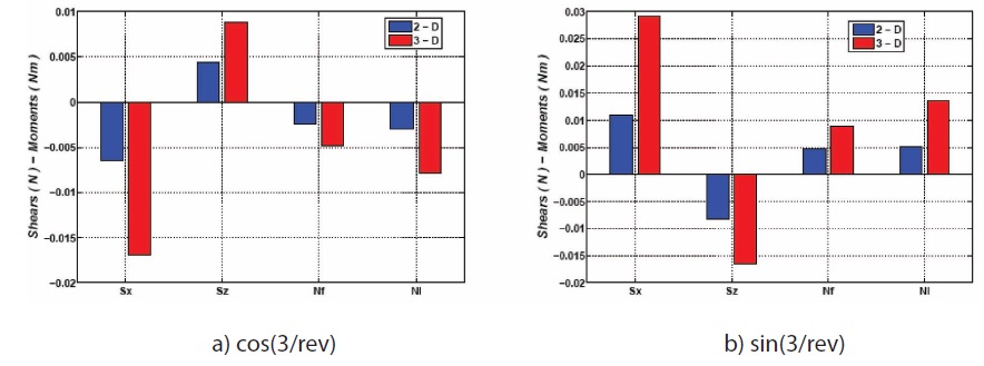
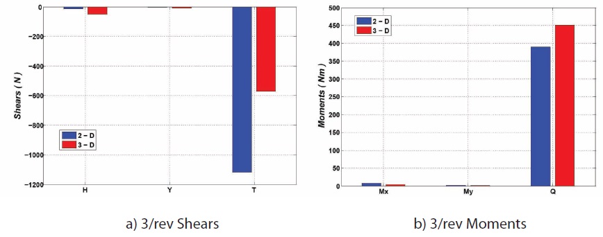
The different evaluations of the static loads are reported in Fig. 23, whereas Fig. 24 refers to the 3/rev harmonics loads.
For the lateral equilibrium, the rotor forces H, Y and the moments Mx, My should be approximately zero; indeed this is the case as represented in Fig. 23. It appears that the 2D and 3D aerodynamic models predict dissimilar results, in particular between the force T and moment Q, being the value of the 2D model greater than the one of the in 3D model. The different evaluation of the dynamic loads leads to an over estimate of the 2D static thrust with respect to the one predicted by a 3D analysis. This fact could be of great interest in designing the windmill tower since the resulting bending moments, evaluated at the basement of the tower, are significant different, i.e., the 3D simulation provides lesser stressed tower structure than the 2D analysis. Furthermore, the 3D analysis predicts a value of moment Q that is greater than the correspondent 2D value, resulting in the capability of the windmill turbine to extract higher power.
Unsteady aerodynamics and aeroelastic characteristics of a medium-sized wind-turbine blade operating under ideal conditions have been considered. The tapered/twisted blade was designed to operate on a stall-regulated downwind wind turbine originally studied in an experiment setup at the NREL. The structural dynamics of the flexible wind-turbine blade has been described by a nonlinear flap-lag-torsion slenderbeam differential model. The aerodynamic quasi-steady forcing terms needed for the aeroelastic governing equations
have been predicted through a strip-theory based on a simple 2D model, whose pertinent aerodynamic coefficients have been obtained using CFD. Aerodynamic loads are computed by CFD and analytical techniques. Turbulence effects in the 2D simulations run for validation purposes were accounted by the Wilcox


![Comparison of the experimental and computational pressure coefficient distribution on the airfoil for the conditions as in Wolfe and Ochs [20].](http://oak.go.kr/repository/journal/12072/HGJHC0_2013_v14n1_30_f006.jpg)