Since Nye and Berry first found dislocations in optical fields in 1974 [1], singular optics have been a subject of interest. The diverse singular patterns provide rich information about the fine structure of light. While phase singularities (wave dislocations, or optical vortices) are frequently encountered in the interference of scalar waves, they resolve into polarization singularities (PSs) when the vector nature of light is retained [2-6]. PSs include C-points (points where the light is circularly polarized) and L-lines (lines where the light is linearly polarized) [2]. These PSs determine the distribution of polarization ellipses around them, such as how in nonparaxial fields the major axes (minor axes) of polarization ellipses surrounding C-points are shown to form Möbius strips [3-5], while in paraxial fields polarization ellipses around C-points produce interesting structures named Lemon, Mon-Star, and Star [2, 6]. Experiments have been successful in generating PSs [7-13], but generation of PSs with a desired shape or structure, especially generation of a Mon-Star, is still a challenge. This is because the distributions of amplitude and phase around C-points are complex and have not been developed clearly.
In this paper, a Cartesian coordinate system with origin at the C-point is established. Then, four curves where the azimuthal angles of polarization ellipses are 0°, 45°, 90°, and 135° respectively are used to determine the distribution functions of amplitude and phase around C-points; these distributions include the Lemon, Mon-Star, and Star. Discussion of these distributions illustrates the difficulty of generating a Mon-Star in experiments. The probabilities of transformation of these three PSs are also discussed. According to the distributions of amplitude and phase, we give suitable functions and simulate several particularly shaped PSs. With the development of modulation techniques for amplitude and phase, it is clear that the work in this paper is helpful for generating arbitrarily shaped C-points in experiments.
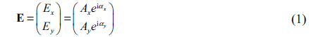
To analyze the distributions of (or constraints for) amplitude and phase around a C-point, we need to write the electromagnetic wave in term of the Jones matrix:

where
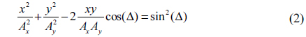
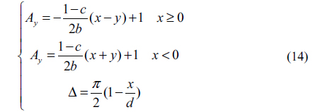
where Δ=
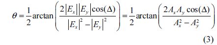
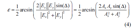
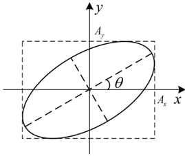
where the azimuthal angle
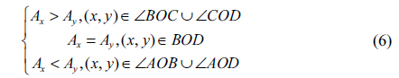
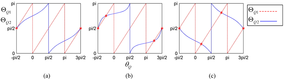
Combining Eqs. (2) and (3) and considering Fig. 1, we obtain the following relationship:
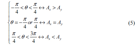
where ↔ is the symbol for “necessary and sufficient”. Eq. (5) is a very important conclusion to determine the distributions of the amplitude and phase difference, as follows.
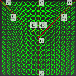
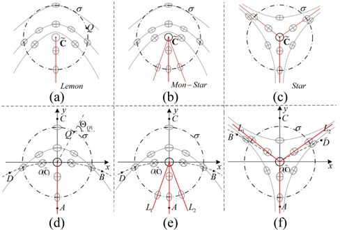
It is well known that there are three typical kinds of polarization singularities: Lemon, Mon-Star, and Star, shown in Figs. 2(a), (b), and (c) respectively [2, 6]. In Fig. 2 the gray ellipses surrounding C-point present the polarization states of the fields. The gray solid curves are the envelopes of the azimuthal angles of polarization ellipses. Among these envelopes, there are some rays (the red rays in Figs. 2(a)~(c)) emanating from the C-points . The azimuthal angles of polarization ellipses on these rays equal the angle between the ray and the +
Next a Cartesian coordinate system is established with origin
Now considering the amplitude distribution of the Lemon in Fig. 2(d), we find the curve

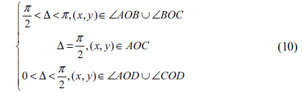
Eq. (6) is the distribution function of amplitude around the Lemon. Now we analyze the distribution of phase around the Lemon. We assume that the field around the C-point is left-hand-polarized, namely 0<Δ<

where
Taking a point that is infinitely close to and on the right of , then the difference in

Eq. (10) means the curve
According to the structures shown in Fig. 2, the ellipses surrounding Lemon and Mon-Star have the same tendency, apart from the number of rays (one for Lemon and three for Mon-Star). In other words, Mon-Star can be regarded as special Lemon. So the amplitude and phase of Mon-Star must be bound by Eqs. (6) and (10), respectively. On the other hand, there exist two other rays and in the field of the Mon-Star, as shown in Fig. 2(e). Naming the azimuthal angles of ellipses on and as and respectively, and implementing the simple transform of Eq. (3), we have
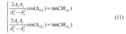
This formula is a function of amplitude and phase simultaneously, which means the amplitude and phase on rays and should follow Eq. (11), while being restricted by Eqs. (6) and (10). It seems complex to construct amplitude and phase that satisfy Eqs. (6), (10), and (11) simultaneously. However, when the amplitude is set according to Eq. (6), the phase can be determined according to Eqs. (10) and (11). Similarly, a set phase can used to determine the amplitude according to Eqs. (6) and (11).
Compared to Lemon and Mon-Star, the Star has a different elliptic tendency. However, the analysis method used above is also suitable for acquiring the distributions of amplitude and phase around the Star. Compared to those for Lemon, the amplitude and phase of Star have the same expressions as Eqs. (6) and (10), respectively, but we emphasize that because of the opposite spatial positions of and in Figs. 2(d) and (f), the distribution of phase for Star differs from that for Lemon. As for Mon-star, there are also two other rays ( and ) in the field of Star, so the amplitude and phase of Star are likewise restricted by Eq. (11).
Now we see that the analyses of amplitude and phase for Lemon, Mon-Star, and Star become very concise. In addition, these distributions of the three PSs can be expressed by the same forms (Eqs. (6), (10) and (11)). These are the benefits of establishing the Cartesian coordinate system and the four rays , , , and .
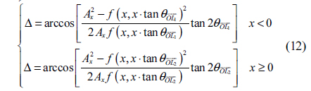
Developing distribution functions of amplitudes and phases around C-points ultimately benefits the generation of PSs. According to the constraints, constructing amplitude and phase is a crucial step in generating the desired PSs. Constructing amplitude and phase functions following Eqs. (6) and (10) for Lemon is easy. Here we try to give expressions used to generate Mon-Star and Star when and coincide with −

Eq. (12) is not the only expression that makes the amplitude and phase obey Eqs. (6), (10) and (11) simultaneously.
In section II we obtained distributions of amplitude and phase around the C-points Lemon, Mon-Star, and Star. We note that the work of [7] is a theoretical description of optical beams carrying isolated polarization singularity C-points. The PSs are formed by the superposition of a circularly polarized mode carrying an optical vortex and a fundamental Gaussian mode in the opposite state of polarization. By varying two parameters, C-points including asymmetric Lemon, Mon-Star, and Star can be generated. Compared to [7], in this paper the electromagnetic waves are written in the more general terms of the Jones matrix, i.e. PSs are formed by the superposition of two linearly polarized modes that are orthogonal to each other. We analyze distributions of the amplitude and phase differences of the two polarized modes. According to the analyses, all three kinds of PSs can be generated (as shown in section IV). Moreover, the positions of the curves where the azimuthal angles of polarization ellipses are 0°, 45°, and 135° can be controlled.
For the Lemon, the amplitude must follow Eq. (6), while the phase must follow Eq. (10). These two formulas are independent constraints on the amplitude and phase, respectively. Thus there is a high probability to obtain amplitude and phase obeying Eqs. (6) and (10), which means generation of Lemon is relatively easy in experiment, such as the interference field of vector waves. As described above, MonStar is a special Lemon for which amplitude and phase are also restricted by Eq. (11), when following Eqs. (6) and (10) respectively. Eq. (11) is a function of both amplitude and phase, which means sophisticated control over phase (or amplitude) is needed to generate Mon-Star. However, in previous studies aiming to generate PSs [8-13], there has been almost no purposeful control over amplitude and phase around C-points. More constraints on amplitude and phase also illustrate that there exists a smaller probability to generate Mon-Star than Lemon in experiments. As Mon-Star, the constraints for generating Star imply that it is also very rare. However, in many studies, fields with Stars are very common.
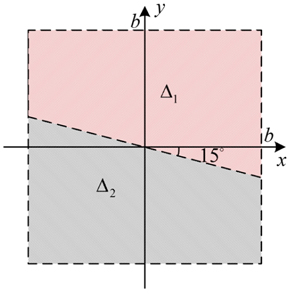
To explain this phenomenon, we consider a point
Now we have seen that Eqs. (6) and (10) are necessary conditions for generating Lemon. Lemon can transform into Mon-Star while the amplitude and phase also follow Eq. (11). For generating Star, Eqs. (6) and (10) are also necessary conditions, while Eq. (11) is not. According to Eqs. (6) and (10) and Figs. 2(d) and (f), the amplitudes of Lemon and Star have the same distribution, while the phase differences have opposite distribution trends. Thus Lemon (Star) can transform into Star (Lemon) if the phase difference of light is modulated by transmission media, such as anisotropic media or a spatial light modulator (SLM).
The purpose of this section is to simulate some specific PSs, such as and with given values. The construction of amplitudes and phases according to sections II and III is a crucial step in generating the desired PSs. We consider the polarization ellipses in a cross section of dimensions 2
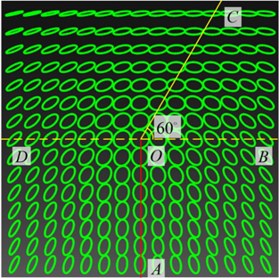
For generating the Lemon, the simplest case is when , , , and coincide with −

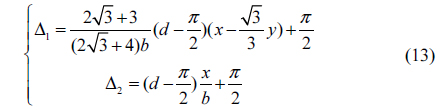
where . Although Δ1 and Δ2 have different expressions, we emphasize that they are equal to each other at the boundary
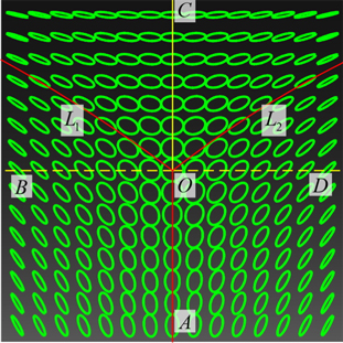
To generate Mon-Star, we can set the amplitude as
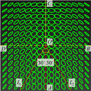
We know that the two conditions of Eqs. (6) and (10) determine the generation of a Star, while another formula, Eq. (11), is needed to generate a specific Star. Figure 7 is a Star with
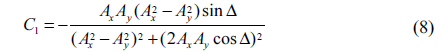
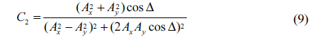
There is a special case, namely that of and , in which Eq. (11) can be rewritten as

where
By establishing a Cartesian coordinate system with origin at a C-point, and with the help of four curves where the azimuthal angles of polarization ellipses are 0°, 45°, 90°, and 135°, the distributions of amplitude and phase around C-points are analyzed and given. We also discuss the necessity of these constraints, which illustrates that there exists a smaller probability to generate Mon-Star than to generate Lemon or Star in experiments. The transformations of these three PSs are also discussed. Suitable modulation of phase difference can make Lemon (Star) transform into Star (Lemon). Compared to [7], PSs with desired shapes can be generated using the constraints obtained in this paper. According to constraints on amplitude and phase, we construct suitable functions and simulate several particularly shaped PSs. These simulations certify the correctness of the analysis and discussions. With the development of modulation techniques for amplitude and phase, it is clear that the distributions of amplitude and phase around C-points are helpful to generate arbitrarily shaped C-points in experiments.