One important aspect on ageing management of nuclear power plants (NPP) is the monitoring and assessment of thermal fatigue [1]. The strong linkage of the long-term degradation mechanism to actual plant conditions, rather than to design assumptions, reveals that its evaluation is a key issue of on-going safety assessments. Thermal fatigue damage and fatigue usage factors need to be carefully monitored and evaluated to ensure continuous safe and economical operation of ageing components and structures.
However, the Civaux 1 failure and comparable incidents reveal that certain piping system Tee connections are exposed to thermal fatigue arising from low- and highcycle temperature turbulences. Inservice experiences show that thermal fatigue cracks may occur arbitrarily in different locations, e.g. welds, base material, straight pipes, elbows, and under rather different loading conditions. These cracks are usually explained by thermal stratification and temperature mixing effects caused by different mass flows in “run” and “branch” pipes at the Tee-connection.
Potential consequences are surface stresses, crack initiation, stresses in the wall or crack propagation. Even though this problem is well known, high cyclic phenomena may not be properly detected by common thermocouple instrumentation and, thus, integrity evaluations rely on estimations and boundary conditions. These approximations may not cover the entire loading conditions and material behavior and, therefore, lead to either too conservative or to not conservative results. Both ways are not acceptable for applications on NPPs, i.e. current fatigue assessment methods have to be adjusted to cover this specific thermal fatigue issue. In particular, the determination of lower not fatigue relevant threshold values in terms of temperature differences, is important for practical plant related applications.
The European Commission funded the international project “thermal fatigue evaluation of piping system Teeconnections” which was launched as a 3-year project with the main objectives to advance the accuracy and reliability of thermal fatigue load determination in engineering tools and to formulate research oriented approaches to outline a science based practical methodology in managing thermal fatigue risks [2].
Therefore, in this study the thermal fatigue evaluation of piping system Tee-connections is performed using fluid-structure interaction (FSI) analysis, addressing the present demand on optimized and verified application procedures for assessing the integrity and safety of Teeconfigurations in safety relevant NPP-systems sustained to significant turbulent thermal stratification and temperature mixing effects. The results will supply valuable information for plant operations and ageing management by improving the confidence in integrity assessments of relevant components, leading to advanced system surveillance with a consequent reduction of operator dose and to an improved cost effectiveness of the NPP.
Turbulent mixing of hot and cold water is characterized by rapid and highly irregular fluid motions. These fluctuations will increase the transfer of energy and momentum as well as the heat convection transfer rate. Turbulence is associated with random fluctuations and the fluid motion occurs on several length scales. Generally, this makes the fluid motion extremely difficult to describe in detail. In the context of turbulent or mixing the description of eddies are used. Eddies are small portions of fluid in irregular motion that exists for a short time before losing its identity. The temperature fluctuations near the pipe wall can be of the order of up to several Hz.
In turbulence the inertia forces are high in comparison to the viscous forces in the fluid. A common measure for this relation is the dimensionless Reynolds number. High Reynolds numbers will indicate higher levels of turbulence in comparison to organized laminar flow. The Reynolds number can be seen as a measure of the ratio between inertial forces and viscous forces. As a rule of thumb, Re > 2000 can be used as a criterion for the onset of turbulent flow in a pipe.
Several recent studies have considered damage due to thermal fatigue in light water reactor components, with a particular focus on those cases resulting in leakage. The NESC failure database could be employed to examine the parameters governing thermal fatigue in nuclear components [3].
The failure cases examined essentially fall into two groups, as observed in other thermal fatigue studies [4]. In the first group the loading is characterized by turbulent mixing (or striping), with or without stratification. Typical components affected by this process are tees without internal mixers. It is noted that none of the through wall cracking cases can be attributed to turbulence alone. However, the observed damage is not just superficial, and cracks penetrating to more than 50% of the wall thickness were observed in a few cases. In the second group the thermal loading is predominantly stratification. Damage caused by stratification appears much more likely to cause leakage, and almost all the cases of through-wall cracking referred to in the present report are associated with this phenomenon. The damage occurs at much lower flow rates than in the turbulent case. The combination of a low flow rate in at least one of the fluids and a high temperature difference controls the damage evolution. It is clear that different forms of stratification exist, the most harmful being the case with a moving interface between a stratified and a non-stratified state.
No case of component rupture was found and any crack growth seems to have been stable up to the point it was detected.
A shutdown cooling system is connected to the reactor coolant system in parallel to eliminate the decay heat during plant shutdown, taking coolant in the hot leg and circulating it into the cold leg. This system for Ulchin 3 and 4 starts to operate when the coolant temperature is 177℃ and its pressure is 3 MPa until the temperature becomes 60℃ with a cooling rate of 41.7 ~ 16.7℃/hr.
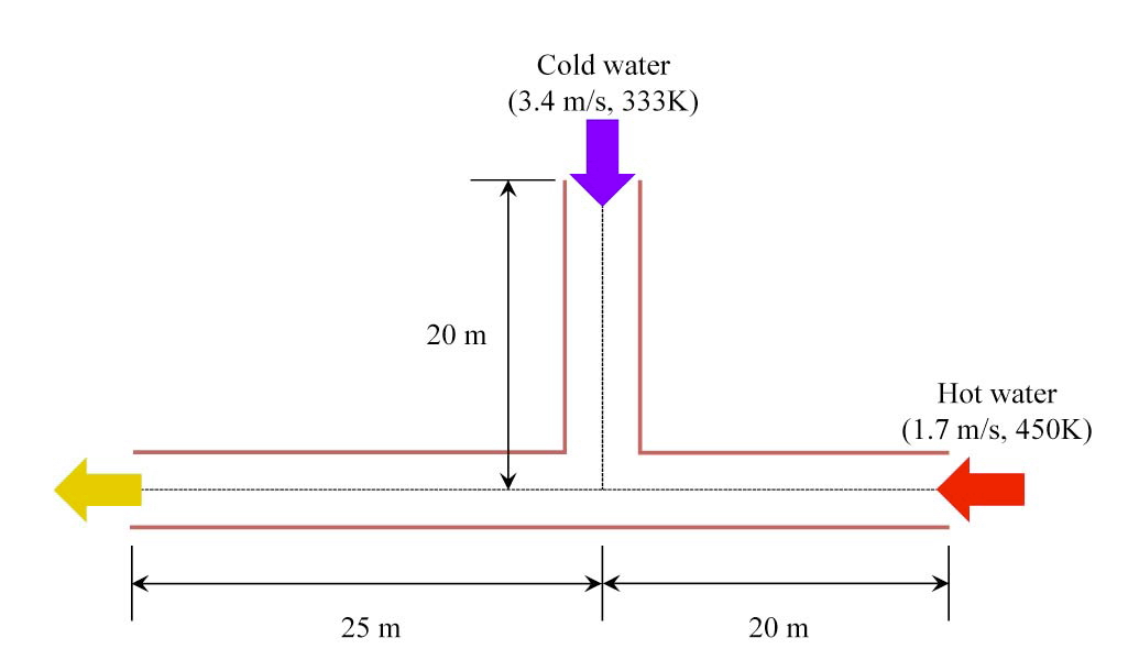
The area to be analyzed in this study is the mixing tee area where the main pipe conveying high temperature coolant meets the branch line pipe carrying low temperature coolant passing through the heat exchanger (Figure 1). In this area, the thermal fluctuation and/or stratification appears due to the high-low temperature mixing flow, which causes thermal fatigue.
The dimensions and operating conditions considered in this study are summarized in Table 1.
[Table 1.] Dimensions and Operating Conditions
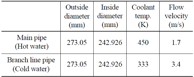
Dimensions and Operating Conditions
3.1 Thermal Hydraulic Analysis
Computational fluid dynamics (CFDs) can in principle be used to compute the flow in a component and thus predict the thermal load. However, if one wishes to fully model turbulence at all length scales (using the so-called direct numerical simulation), a computational time is excessive even with current processing performance. Therefore, several alternative modeling strategies have been developed, with the Reynolds Averaged Navier- Stokes (RANS) approach being the most widely used. Its advantage lies in a simple model and numerical formulation. On the downside, RANS does not resolve the turbulent spectrum and provides only limited information on unsteady mixing processes [5].
In recent years, an intermediate approach called the Large Eddy Simulation (LES) is being increasingly applied. LES aims at resolving all large scales in the flow domain. Only small (dissipative) structures are modeled by the subgrid scale eddy viscosity. The advantage of LES is that only a small portion of the flow is modeled, whereas most of the turbulence is a result of the numerical solution of the unsteady-state, three-dimensional Navier-Stokes equations. A disadvantage is that LES is computationally more expensive than the RANS approach.
In order to determine thermal load in a mixing tee, the use of LES is imperative. The RANS approach simply does not provide enough detailed information. On the other hand, thermal stratification problems e.g. in elbows, can still be evaluated accurately with RANS.
Using ANSYS CFX 13.0 [5], a thermal hydraulic analysis is performed for the piping system with mixing tee junction. The fluid region inside the pipe is modeled by the ANSYS Design Modeler. The transient analysis is performed for 300 seconds with a time step of 0.1 seconds.
Considering the density variation of fluid with respect to the temperature, the momentum equation is
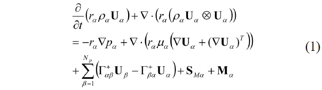
where S

where the density difference
Generally, a full buoyancy model or a Boussinesq model is used to apply a momentum source due to density differences. However, the Boussinesq model can’t represent density as a function of pressure or temperature. Therefore, in this analysis a full buoyancy model is used to consider the density difference.
A total energy effect is considered along with the full buoyancy condition to simulate the thermal stratification more accurately, because Equation (3) can consider conduction, convection and also viscous work due to turbulence.

where
In a tube Reynolds number is defined as

where
In the past,
This study aims to develop a thermal fatigue assessment methodology rather than to get the exact solution and therefore the SST model is used instead of the LES model, which has the advantage of accurate simulation of turbulence and the disadvantage of mesh generation and solving time.
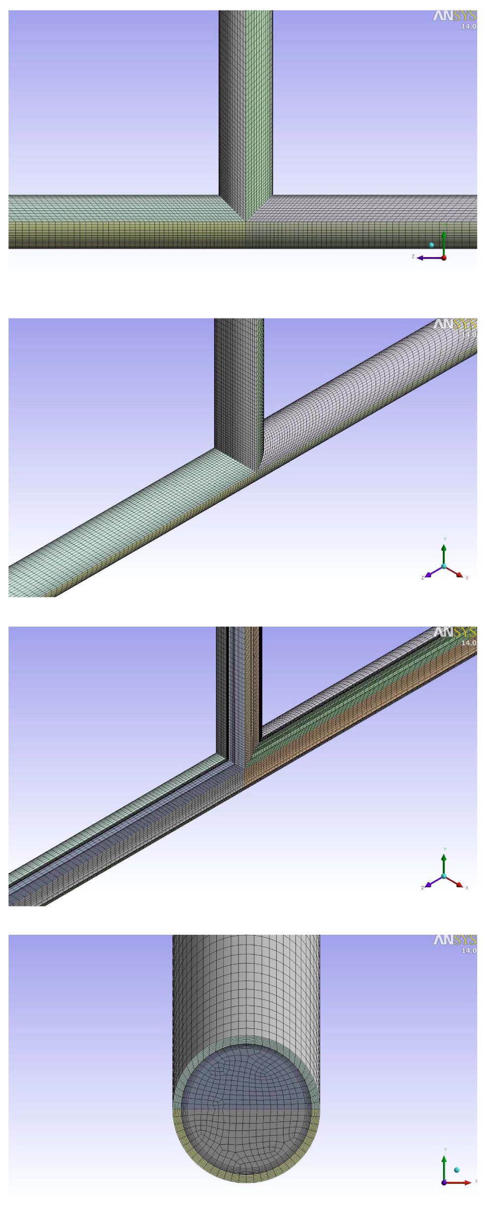
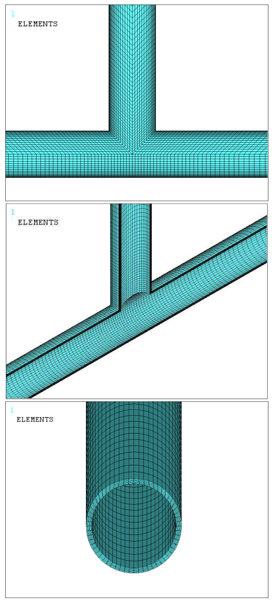
A hexagonal mesh with about 540,000 elements is generated as shown in Figure 2. The number of nodes is determined based on the sensitivity study to increase the accuracy of the solution.
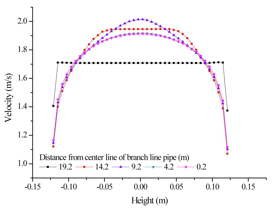
A sufficient length of pipe is included in the model to develop the flow fully as shown in Figure 3. The results of the sensitivity study show that a length of 20 meters in the upstream of the main piping system is sufficient for the fully developed flow.
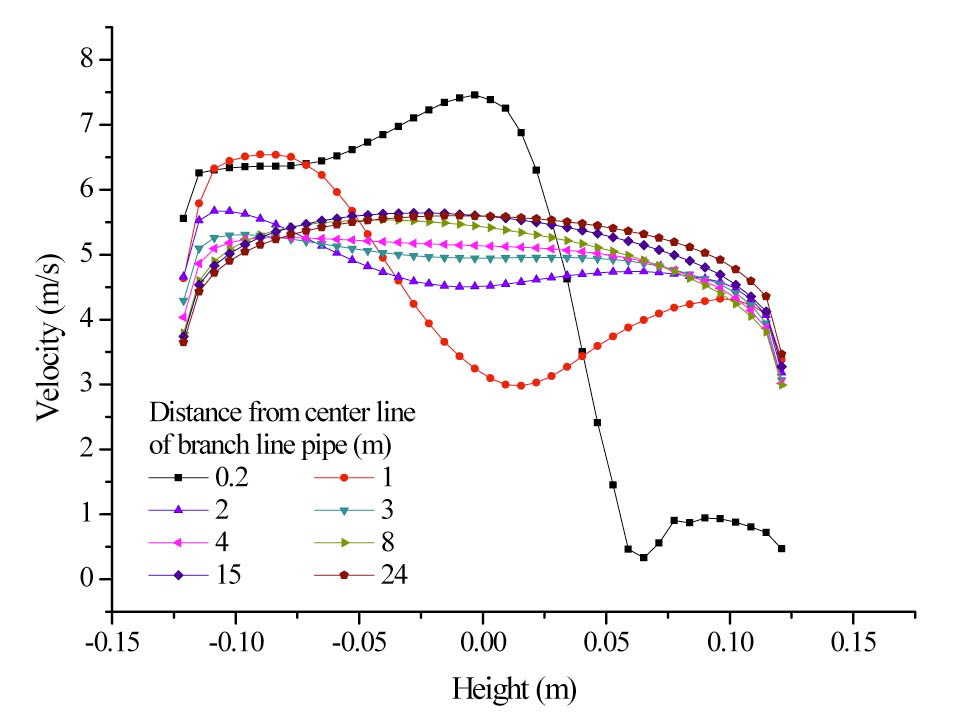
The flow profile of the downstream is shown in Figure 4, which shows that the velocity changes at the junction are significant but the flow tends to remain stable at the outlet region.
3.2 Stress and Fatigue Analysis
The stress analysis is performed to get the thermal stress distributions in the pipe using the finite element model taken directly from the CFX model as shown in Figure 5. The model uses 3-dimensional 8-node structural solid elements (SOLID185) and it has 560,341 nodes and
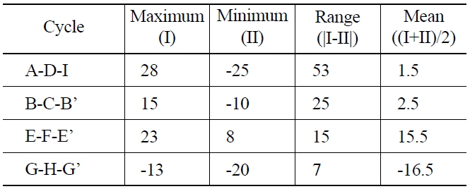
[Table 2.] Summary of Cycle Countings

Summary of Cycle Countings
543,180 elements [6]. The fixed boundary conditions in the axial and circumferential directions are applied at inlet ends of the pipe and no axial movement at the outlet location is applied.
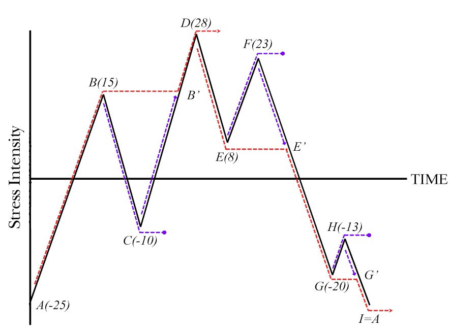
Fatigue analysis of the mixing tee is performed for which rain flow method of cycle counting is used. The alternating stress in the rain flow method is determined as in Table 2 for the stress history of Figure 6 [7,8].
A design fatigue curve is used to determine the usage factor for austenitic steel [9].
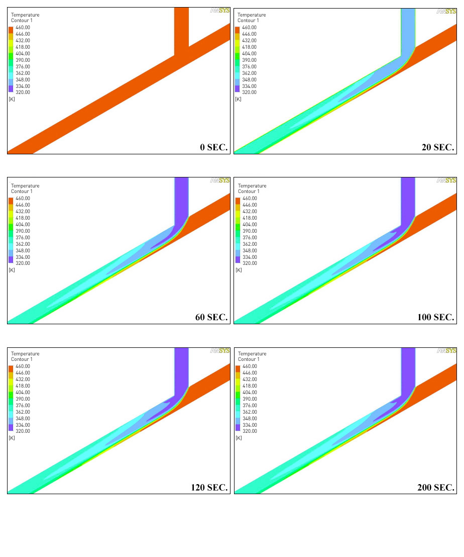
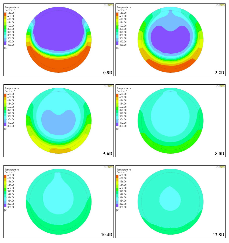
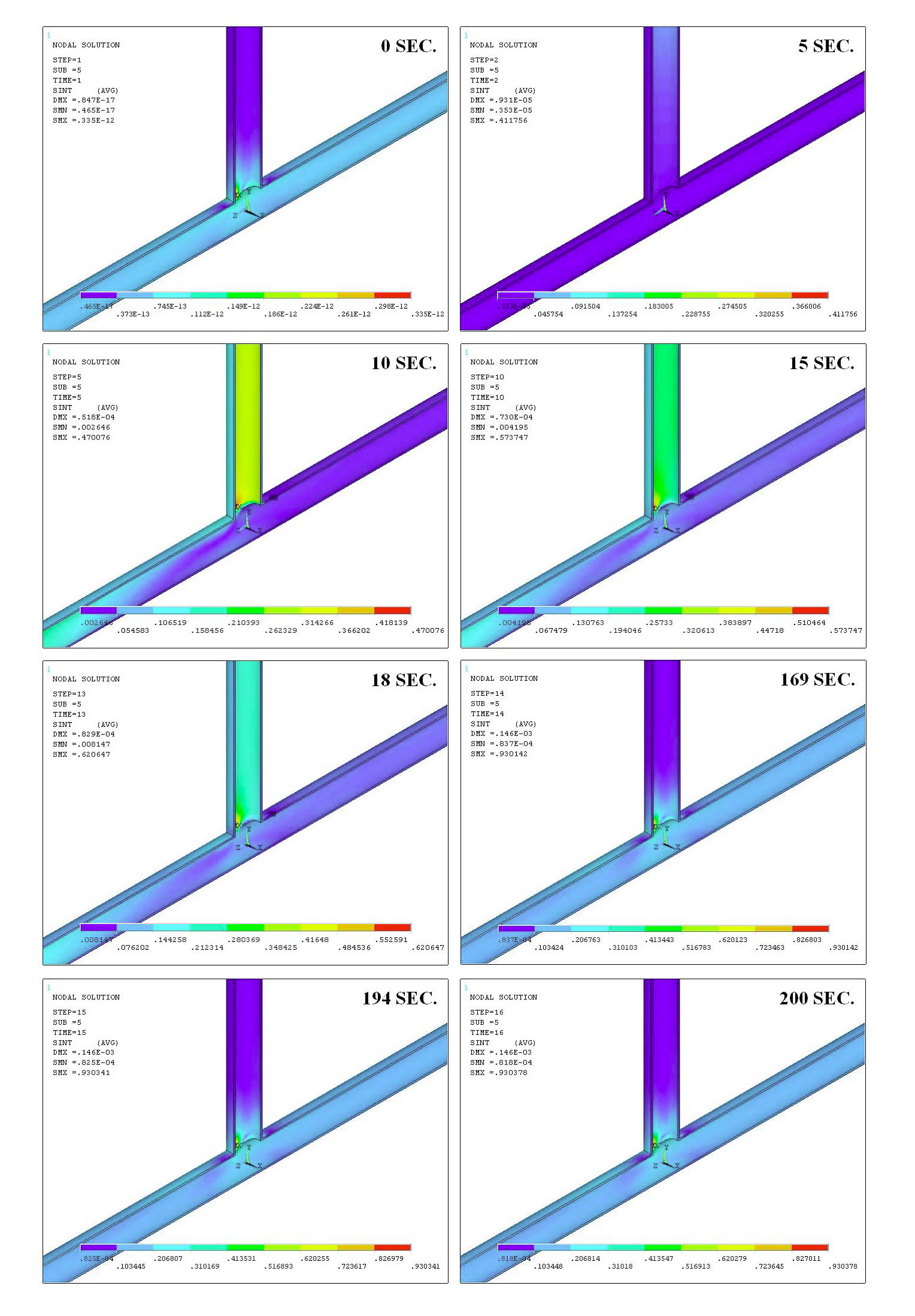
Figure 7 shows the transient temperature distributions at the wetted wall surface at several elapsed times after the beginning of mixing flow. Figure 8 displays the transient temperature distributions at several cross-sections of the main pipe down stream at the elapsed time of 100 seconds after the beginning of the mixing flow.
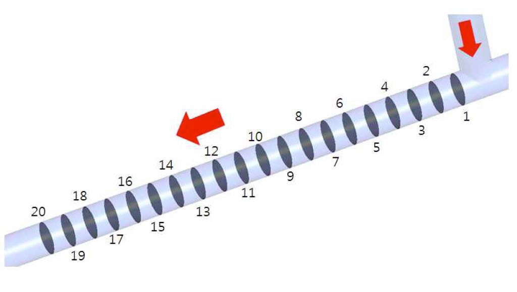
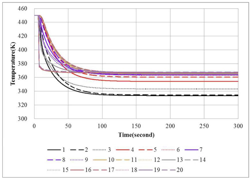
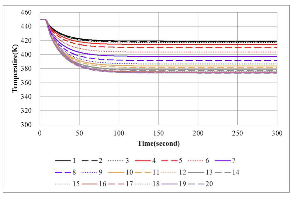
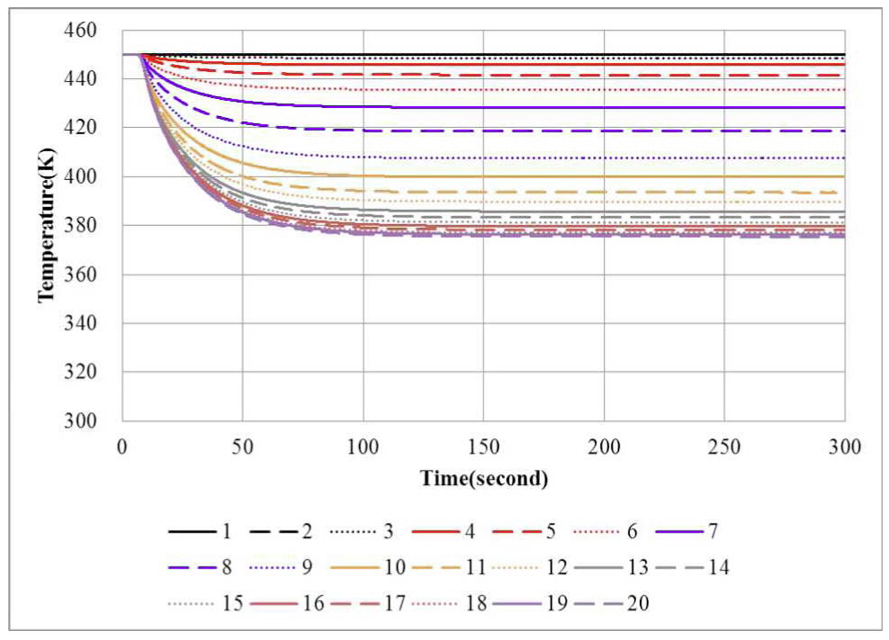
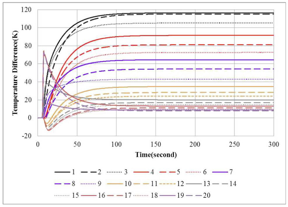
The temperature histories of three points at the 20 locations along the main pipe in Figure 9 are plotted as shown in Figures 10 through 12. The comparisons between three points show that the temperatures at the top point are lowered more rapidly than those at the bottom point, which means that there exists thermal stratification as shown in Figure 13. Also it is found that the stable temperatures for all locations are obtained at about 100 seconds after the mixing flow begins.
The stress analysis is performed to get the thermal stress distributions in the pipe using the finite element model taken directly from the CFX model. Temperature distributions of the pipe obtained from the thermal hydraulic analysis are used as an input to the structural analysis to get the thermal stresses as shown in Figure 14. In addition they are used to calculate fatigue usage factors.
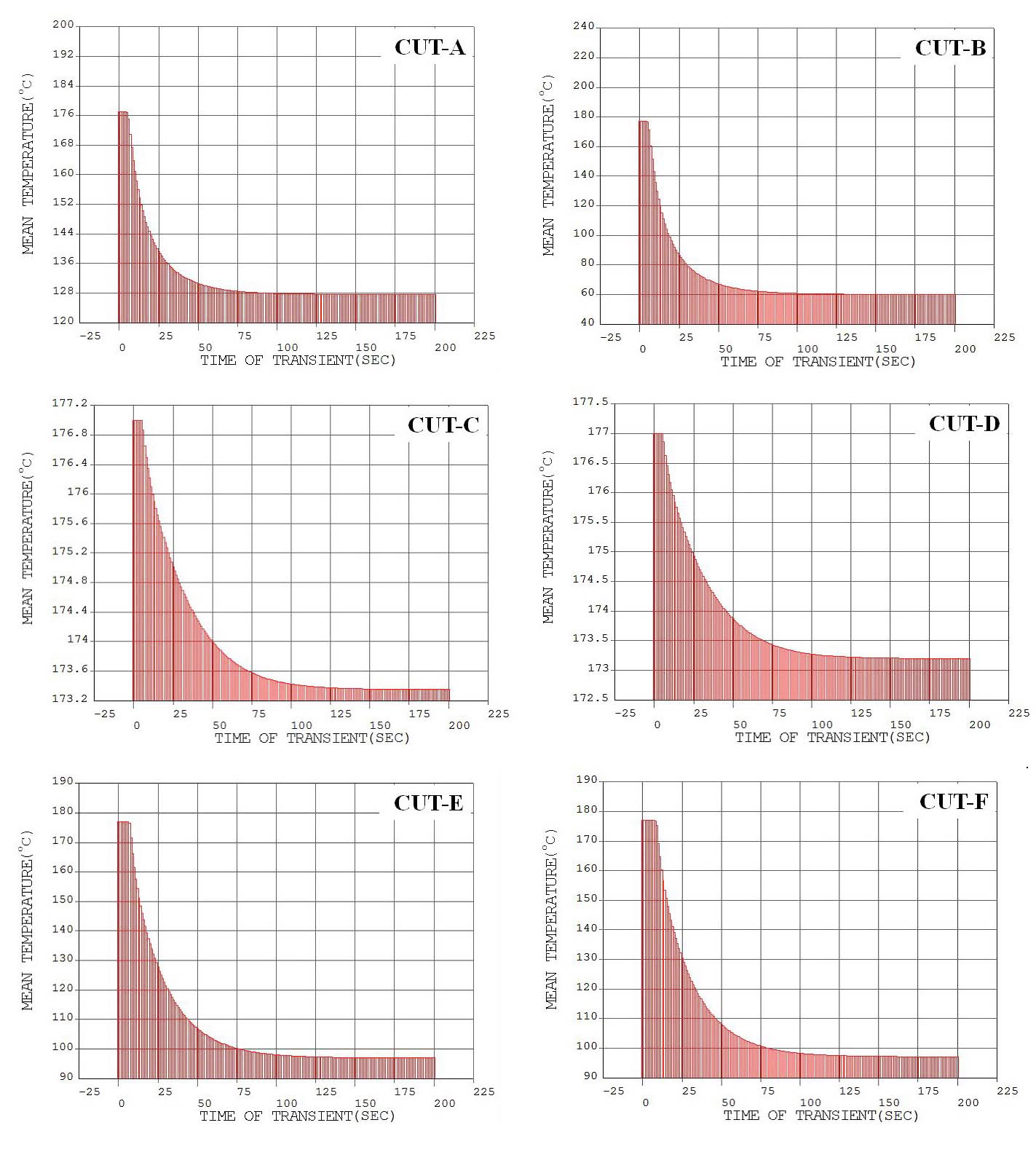
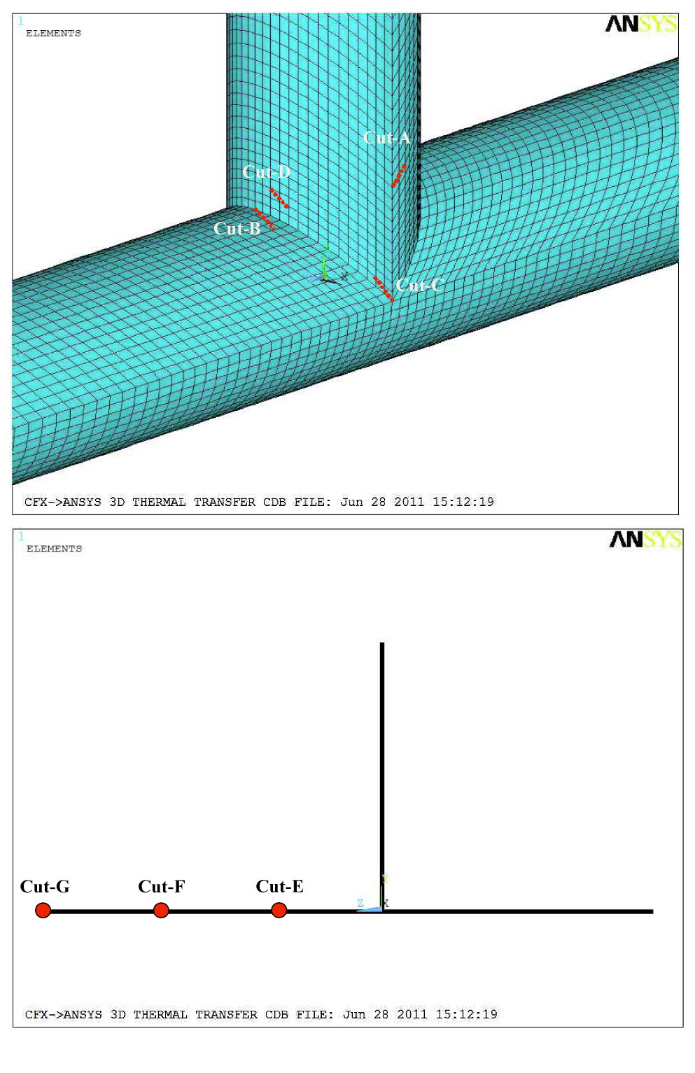
Seven cuts are chosen from experience for calculating the fatigue usage factors as shown in Figure 15. Cuts from A through D are located at the junctions of mixing tees and cuts from E through G are located at the 1/3 locations of the down stream in the main pipe.
[Table 3.] Fatigue Usage Factors for Selected Locations
Fatigue Usage Factors for Selected Locations
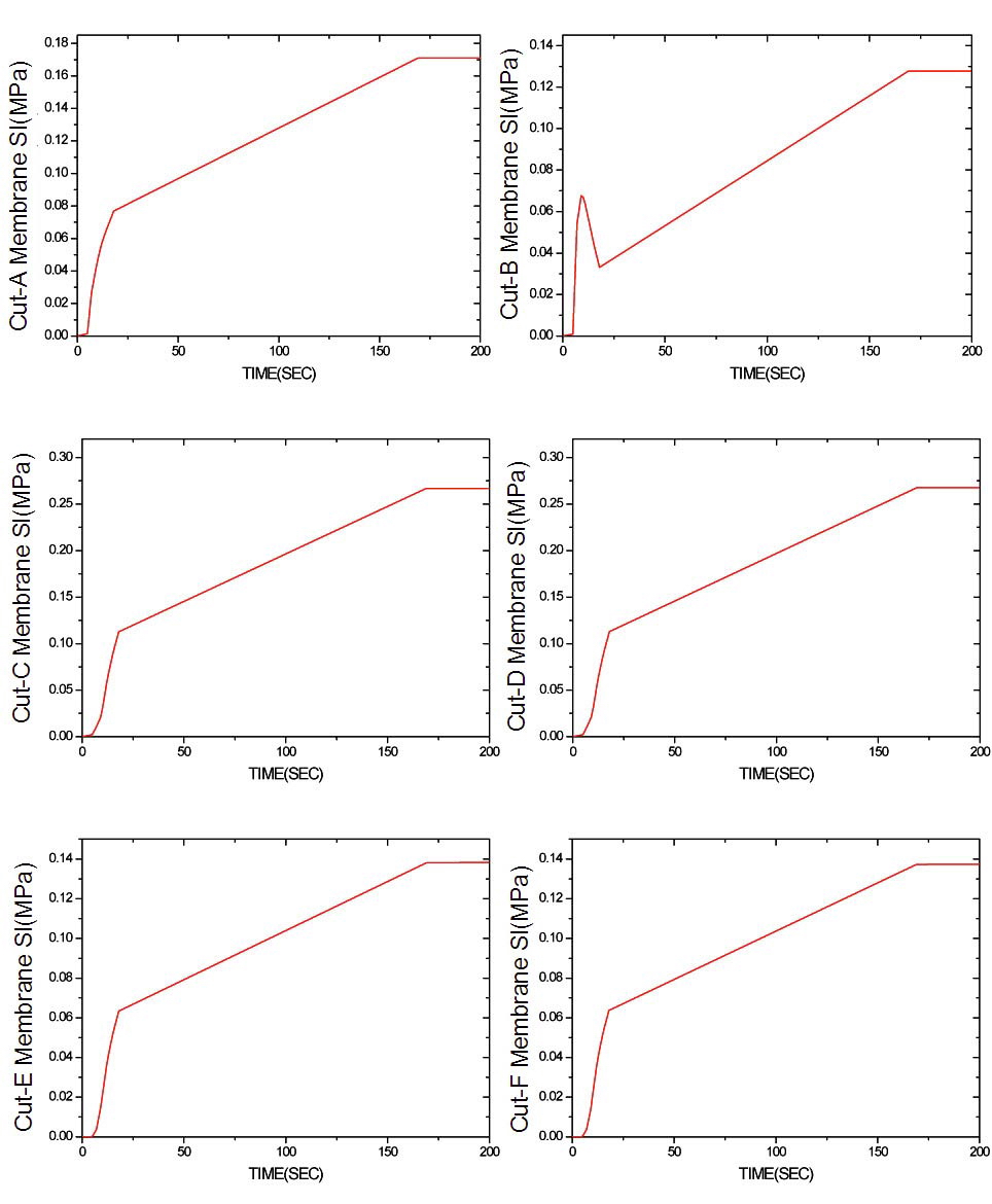
The mean temperature variation at each cut is shown in Figure 16, which shows that it is almost uniform after 170 seconds from the starting point when mixing flow begins. In the same way, the equivalent stress variation at each cut is shown in Figure 17, which also shows that it is almost uniform after 100 seconds as expected.
The fatigue usage factors calculated at inside and outside of the cut points for the cycles of 5.8E10 are summarized in Table 3. The usage factors are almost the same for all locations because the stress intensities due to thermal
mixing are almost negligible and the allowable numbers of cycles from the design fatigue curve are almost the same for all locations.
The procedure for improved load thermal fatigue assessment using FSI analysis is suggested in this study to supply valuable information for establishing a methodology on thermal fatigue.
A detailed CFD analysis involving conjugate heat transfer analysis is performed to obtain the transient temperature distributions in the wall of the mixing tee subjected to a high-low temperature mixing flow during plant shutdown using a commercial CFD code. The thermal loads from CFD calculations are transferred to ANSYS Multiphysics which is employed for the thermal stress analysis. From the thermal stress analysis, the response characteristics of the T-junction subjected to the mixing flow are investigated, and the fatigue analysis is ultimately performed. Using the rain flow method for cycle countings, fatigue usage factors are calculated for locations concerned and are found to be very low.