A failure detector is a key building block for fault-tolerant distributed system, which provide a mechanism to collect information of process failure. Chandra and Toueg [1] introduced the concept of an unreliable failure detector and many fault-tolerance algorithms have been proposed based on unreliable failure detectors.
Recently, some adaptive failure detectors have been presented [2-6]. Most of them are based on a heartbeat strategy and modify the timeout value dynamically according to the network conditions. Chen et al. [7] estimate (hereinafter, Chen’s estimation) the next heartbeat arrival time by computing the average transmission time and a fixed safety margin is added. Bertier et al. [8] combine Chen’s estimation and a dynamical safety margin based on Jacobson’s [9] estimation of the round-trip time.
In addition, some studies [10-12] introduce Omega failure detectors (type of failure detectors) which judge process failure not according to the check point, but according to an output value φ (0 ≤ φ ≤1) in order to present the reliability of the process.
The next part of this section will introduce the failure detector properties and the quality of service of the failure detector.
>
A. Failure Detector Properties
Failure detectors are characterized by two properties: completeness and accuracy. Two kinds of completeness and four kinds of accuracy are defined [1, 13].
Completeness characterizes the failure detector's capability to suspect every incorrect process permanently. Two kinds of completeness are defined.
1) Strong completeness: Eventually, every process that crashes is permanently suspected by every correct process. 2) Weak completeness: Eventually, every process that crashes is permanently suspected by some correct process.
Accuracy is the characterization of the failure detector’s capability not to suspect correct processes. Four kinds of accuracy are defined.
1) Strong accuracy: No process is suspected before it crashes. 2) Eventual strong accuracy: There is a time after which correct processes are not suspected by any correct process. 3) Weak accuracy: Some correct process is never suspected. 4) Eventual weak accuracy: There is a time after which some correct process is never suspected by any correct process.
Eight classes of failure detectors are yielded by combining the two kinds of completeness and four kinds of accuracy, named as perfect,
Generally speaking, a good failure detector should be a
>
B. Quality of Service of Failure Detectors
Some metrics have been proposed to specify the quality of service of a failure detector [14]. The main metrics are as follows:
● Detection time: The time from when the process crashes to the time when it is permanently suspected. ● Mistake recurrence time: The time between two consecutive mistakes. ● Mistake duration: The duration time for the failure detector to correct a mistake.
The rest of this paper is organized as follows: Section II describes our failure detection model; Section III presents the new algorithm in our failure detector; Section IV proves that it is an eventually perfect failure detector; Section V presents the performance evaluation by a series of experiments; and Section VI consists of the conclusion of our research.
Ⅱ. THE MODEL OF FAILURE DETECTION
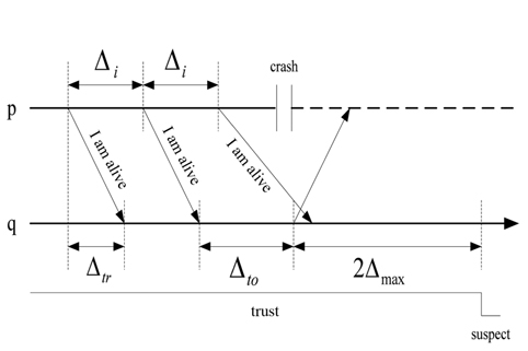
The heartbeat model [15] is used in most distributed systems. Every process
If
The heartbeat interval Δ
The process
>
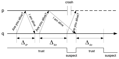
C. The Dual Model of Heartbeat and Interaction
In this paper, we will use a dual model of heartbeat and interaction. The dual model is organized in two steps. First, the heartbeat model is used to detect the process failure. If a process
Ⅲ. AN EXPONENTIAL SMOOTHING ADAPTIVE FAILURE DETECTOR
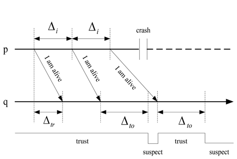
Chen’s estimation is a classical adaptive failure detector algorithm. It estimates the arrival time of the next heartbeat message according to the historical time sequences of the heartbeat messages. In addition, a constant safety margin is added to raise the detector’s accuracy.
The process
The timeout checking point is
where is ∂ the constant safety margin.
Chen’s failure detection algorithm can estimate the arrival time of the next heartbeat message dynamically. However, it uses a constant safety margin, and the suitable constant ∂ is difficult to determine in a condition with a complex network. In addition, the algorithm uses the average transmission delay of the most recent
An improved estimation algorithm based on exponential smoothing is proposed to overcome the shortcomings of the base algorithm. Exponential smoothing [16] is a technique that can be applied to a time data sequence. It makes forecasts according to a series of historical data.
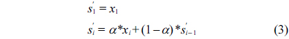
The delay data sequence is represented by {
where α is the smoothing factor, and 0 < α < 1.
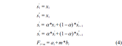
The above simple exponential smoothing does not perform well when there is a trend in the data. In such situations, double exponential smoothing is used to estimate the following data in a sequence with a linear trend. Double exponential smoothing works as follows:
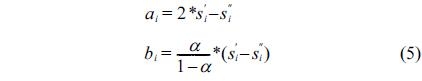
where
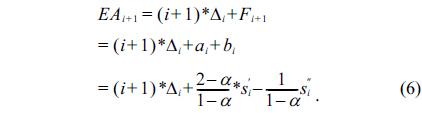
Then,
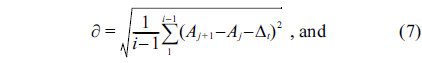
Another improvement in the algorithm is that the dynamic safety margin is calculated using the mean square deviation. As shown in Fig. 1, if the two adjacent heartbeat messages have the same transmission delay, then,
Finally, we have
Algorithm 1 is the exponential smoothing adaptive failure detector (ESA_FD) algorithm.
Our failure detection algorithm can meet the requirements requirements of class ◇
Theorem 1. Strong completeness.
Every crashed process
∃t0 :∀t ≥ t0, ∀q∈correct(t),∀q∈crashed p∈suspectq(t).
Before providing proof, we defined several parameters:
Δmax: The unknown bound time threshold on the message transmission between processes p and q.mk: The kth message that process p sends to q.tsk : The time when process p sends mk to q.trk : The time when process q receives mk.tc : The time of a crash of process p.
When the process p crashes at
The next thing to be proven is that τ
where
So there is an upper bound (
Theorem 2. Eventual strong accuracy.
Theorem 2 states that there is an upper bound time after which the correct processes are not suspected by any correct process.
∃
However, since the maximum transmission delay is Δmax, the dual model of heartbeat and interaction is used in this paper. In the worst network conditions, the checkpoint isτ
Two computers are used to build the experimental platform in a local area network. One machine runs a program to send heartbeat messages (like process
In the paper, we compare ESA_FD to conventional FD and Chen’s FD. The conventional FD sets a fixed timeout Δ
Chen’s FD estimates the arrival time of the next heartbeat message dynamically and it uses the average transmission delay of the most recent
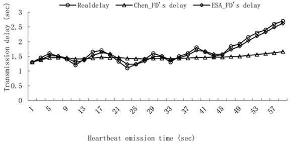
Experiment 1. Transmission delay contrast.
We count thirty transmission times of the heartbeat messages and the heartbeat interval is set to 2 seconds. We compute the transmission delay according to the estimation of the arrival time by using Chen’s FD and ESA_FD. The result is shown in Fig. 5.
Since the average delay is used to estimate the arrival delay in Chen’s FD, Chen’s FD is only suitable for a series of random data and there is a big difference between the real transmission delay and Chen’s estimation when the data has a linear trend. Whereas the estimation in ESA_FD confirms the real transmission delay very well, exponential smoothing uses a weight value to emphasize the recent data and ESA_FD is suitable for the data not only for random but also for linear trends.
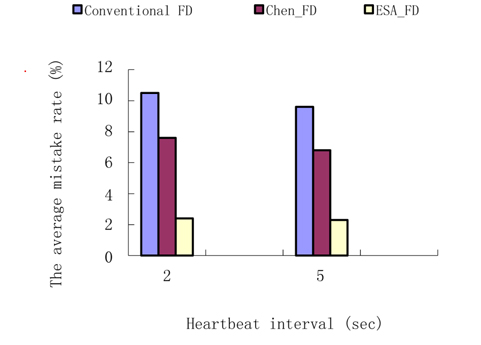
Experiment 2. The average mistake rate contrast.
Two groups of tests are involved in computing the average mistake rate. The heartbeat interval of the first group is set to 2 seconds and the other is set to 5 seconds. The fixed timeout in the conventional FD is set to 1.8 seconds and the safety margin in Chen’s FD is set to 0.5 seconds. The result is shown in Fig. 6.
Since the conventional FD uses a fixed timeout to detect a failure, and it is difficult to choose the fixed value to fit complex network conditions, so the fixed timeout of 2 seconds may not be the most suitable value since it results in a high mistake rate of about 10%. Chen’s FD is better than the conventional FD, but it is not suitable for data with a linear trend. Therefore, the safety margin is an important adjustment for the result, and in the same manner as the conventional FD, it is hard to determine the value of the safety margin. The ESA_FD in this paper has a very low mistake rate providing accurate estimation to the transmission delay and dual detection starts while a process timeouts first. This further raises the accuracy of detection.
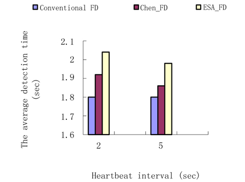
Experiment 3. The average detection time contrast.
The parameters are set as in Experiment 2. In the experiment, we count the detection time and the result is shown in Fig. 7.
EFA_FD uses dual detection while a process is suspected, so it takes more time than Chen’s FD. However, since the estimation to the transmission is more precise, the amount of time for dual detection is shorter, and the difference between the Chen’s FD and ESA_FD is very small. So EFA_FD raises the detection accuracy by increasing detection time by a small margin.
ESA_FD is an improved adaptive failure detector, which is more suitable for complex network conditions than Chen’s FD. On the one hand, ESA_FD uses exponential smoothing to predict the next data and the prediction through exponential smoothing is more accurate than Chen’s prediction, which is calculated with the average value, because Chen’s FD is only suited for random data with little fluctuation. Hence, ESA_FD can more accurately predict the series of data not only for random, but also in linear trends in applications where the weight value is of exponential smoothing. On the other hand, ESA_FD calculates the safety margin with the mean square deviation and it varies dynamically according the historical transmission delay. ESA_FD meets the requirements of strong completeness and eventually strong accuracy and the experimental results show that ESA_FD can increase the accuracy substantially by increasing the detection time by a small amount.