One of the significant issues in multiprocessor scheduling is how to better utilize processors. The scheduling algorithms are classified as global scheduling and partitioned scheduling. In global scheduling, only one queue exists for the entire system, and tasks can run on different processors. This scheduling algorithm has high overhead. On the other hand, in partitioned scheduling, each processor has a separate queue, and each task may only run on one processor.
The problem of partitioned scheduling is very similar to bin-packing, which is known to be NP-hard [1]. In recent years, a new approach called semi-partitioned scheduling has been proposed. In this approach, most tasks are assigned to a single processor, while a few tasks are allowed to be split into several subtasks and assigned to different processors to improve utilization.
The delayed rate monotonic algorithm is a modified version of the rate monotonic algorithm, which can achieve higher processor utilization than the rate monotonic algorithm [2, 3]. In this algorithm, a new state called the delayed state is added to the system. All tasks except for the one with lowest priority enter this state as they make a request. It is proven that the delayed rate monotonic can safely schedule any system composed of two tasks with total utilization less than or equal to that on a single processor.
In this paper, the problem of scheduling tasks with fixed priority on multiprocessor platforms is studied. The proposed approach can increase the utilization of some processors to 100% based on the delayed rate monotonic policy. Our novel contributions are as follows:
First, it is formally proven that any task which is feasible under the rate monotonic algorithm will be feasible under the delayed rate monotonic algorithm as well. Then, we propose a new semi-partitioned scheduling algorithm based on the delayed rate monotonic algorithm called SS-DRM, which adapts a previous allocation method [4] with the delayed rate monotonic algorithm. The scheduling policy [4] is based on the rate monotonic algorithm. The use of the delayed rate monotonic algorithm makes SS-DRM perform better against possible overload compared to the rate monotonic algorithm. After that, two improvements are proposed to change the allocation method of SS-DRM in order to improve the processor utilization by using a new pre-assignment function and a new splitting function. Based on these two improvements, SS-DRM can achieve full processor utilization in some special cases. Another advantage of the new pre-assignment function is the number of created subtasks that can be safely scheduled. The simulation results demonstrate that SS-DRM improves the scheduling performance compared with previous work in terms of processor utilization, the number of required processors, and the number of created subtasks.
The rest of this paper is organized as follows. In Section II, related works are discussed, while in Section III, the system model is introduced. Sections IV and V are related to the allocation method and SS-DRM. Finally, an evaluation and conclusions are discussed in Sections VI and VII.
The first semi-partitioned technique was used with the EDF algorithm for soft real-time systems [5]. Then, some studies worked on periodic tasks [4, 6-8]. An approach called PDMS_HPTS selects and splits the highest priority task in each processor [8]. The scheduler of processors in this paper is based on the deadline monotonic algorithm, with which the utilization is 60%.
In some other research, the processor utilization is raised up to the well-known L&L bound (
Increasing the processor utilization beyond the L&L bound has also been studied in some papers. An approach called pCOMPATS was proposed [6] for multicore platforms. As the number of cores increases, this approach can achieve 100% utilization. When the utilization of each task does not exceed 0.5, this processor utilization is achieved. Therefore, tasks are divided into two groups: light tasks with utilization of lower than 0.5 and heavy tasks with utilization more than or equal to 0.5. Light tasks are assigning by a first-fit method. First, tasks are sorted in ascending order of their periods, and then allocation is done from the front of the queue towards the end. Heavy tasks are assigned like PDMS_HPTS. It means that the highest priority task is selected and then split. The least upper bound to the processor utilization for heavy tasks is 72%.
The scheduler of processors is based on the rate monotonic algorithm, and the schedule-ability test used in this paper is R-bound [11]. This schedule-ability test was proposed by Lauzac et al. [11] in 2003. Their approach is sufficient for the schedule-ability test with good approximation.
The RM-TS approach increases the processor utilization beyond the L&L bound [4]. As in another study [7], the worst-fit method is used in the allocation of RM-TS, but admission control in RM-TS is based on response time analysis, so the processor utilization can be improved. There are also some other works which studied semi-partitioned scheduling based on the earliest deadline first algorithm [12, 13].
The approach of this paper can also increase the processor utilization more than the L&L bound based on delayed rate monotonic policy. The overhead of task splitting is the same as in previous approaches [6, 8]. Based on these studies, the overhead of context switching due to task splitting is negligible. There are also some other approaches that are similar to delayed rate monotonic approach which improves the schedule-ability of the rate monotonic algorithm. This group of scheduling algorithms studied the problem of fixed priority scheduling with a limited-preemptive approach. For instance, an approach was proposed that improves the feasibility of tasks, so the processor utilization could be enhanced [14].
In the proposed system, tasks are periodic, and their deadline parameters (i.e., relative deadline) are assumed to be equal to their periods. A request of task
Ci = the worst-case execution time required by task τi on each job. Ti = the time interval between two jobs of task τi.
Tasks are considered hard real-time (as opposed to soft real-time [3]). Every job of task
Liu and Layland [15] proved that the worst response time of task
DEFINITION 1.
DEFINITION 2.
DEFINITION 3.
A semi-partitioned scheduling includes two phases: partitioning and scheduling. In the partitioning phase, all tasks are assigned to the processors. If a task cannot be entirely accommodated by a processor, it is split into two subtasks. These tasks are called split-tasks. The other tasks which are entirely assigned to a processor are called non-split tasks. Non-split tasks always run on a single processor.
The second phase of a semi-partitioned scheduling is the policy to determine how to schedule assigned tasks on each processor. The scheduler used within each processor is based on the delayed rate monotonic algorithm, which is an improved version of the rate monotonic algorithm [15]. In the rate monotonic algorithm, every task with a lower period has higher priority. Further, this algorithm is preemptive. So, the lowest priority task has the highest probability for overrun. In the delayed rate monotonic algorithm, all tasks have a secure delay except for the task with the lowest priority. Therefore, in this scheduler, these two queues are defined for tasks:
Ready: a task with the lowest priority directly enters this queue, and other tasks enter when their delays are over. Delay: all tasks except for the lowest priority one enter this queue as they make a request.
A task in the ready queue has higher priority over all tasks in the delay queue. If no tasks exist in the ready queue, then a task is selected from the delay queue to run next. Tasks in both ready and delay queues are scheduled based on the rate monotonic algorithm. Suppose tasks are sorted in ascending order of their periods. Now, Formula (3) calculates the delay of each task.
For
For
Parameter
It should be mentioned that the concept of delay used by the delayed rate monotonic algorithm is different from zero laxity [16]. If
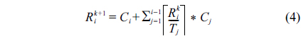
An approach called RM-TS was introduced in another study [4] for allocating tasks on multiprocessor platforms with a semi-partitioned technique and the rate monotonic algorithm. In this paper, the schedule-ability test is based on the response time analysis (RTA) [17]. The worst response time of a task under the rate monotonic algorithm can be calculated by Formula (4). Suppose tasks are sorted in ascending order of their periods. Now, the worst response time of task
This iteration is terminated when then task
EXAMPLE 1. Task set Γ includes three tasks with the parameters shown in Table 1. Now, we want to check whether this task set is schedulable under the rate monotonic algorithm or not.
[Table 1.] Period and worst-case execution time of tasks
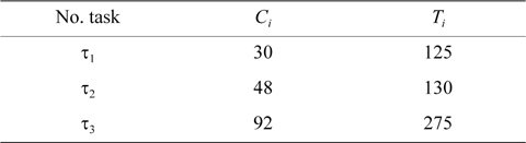
Period and worst-case execution time of tasks
● First,
● Second,
● Third,
The worst response time of all tasks is lower than their periods. Therefore, task set Γ is schedulable under the rate monotonic algorithm.
Tasks in RM-TS are classified into two groups.
● Light: task
● Heavy: task
>
A. Pre-assignment Function for Heavy Tasks
First, tasks are sorted in descending order of their periods, and then a pre-assignment function is done from the end of the queue towards the front. In the pre-assignment function, the heavy tasks which satisfy Condition (5) should be separated and assigned to processors in the preassignment phase. These processors are called pre-assign processors. Suppose
Λ(
After the pre-assignment phase, it is time for the remaining tasks. These tasks are called normal tasks. Based on the sorting method, the lowest priority task is in front of the queue. Now, a processor is chosen among normal processors with the worst-fit method. It means the processor with the lowest load factor is chosen for assigning the current task. If all tasks (including the current task) in this processor can be feasible and all can meet their deadlines, we can add the entire task to this processor. As mentioned, such a task is called a non-split task. If an infeasible task exists, then the current task should be split. This task is called a split-task. The first part is added to the processor, and the second part is put back in front of the queue. After adding the first part to a processor, no other task or subtask is assigned to this processor.
If no normal processor exists, then a pre-assign processor is chosen. In this case, the pre-assign processor which has a task with the largest period is chosen for assigning.
This process continues. If the queue of tasks is empty, we can say that all tasks are successfully assigned to processors. Algorithm 1 shows the pseudo-code of the allocation method of RM-TS.
It is easy to derive the following property from Algorithm 1.
LEMMA 1.
Now, under the rate monotonic algorithm, the first subtask of a split-task will start its execution as soon as it makes a request, and it will run to the end without any interruption. Other subtasks of a split-task should wait until the prior subtasks are completed before starting to execute. For this concept, the term of release time is used [4]. It means that the release time of each subtask of a split-task is equal to the total worst response time of prior subtasks. This release time is calculated as shown in Formula (6).
Suppose task
These subtasks need to be synchronized to execute correctly. For example, subtask cannot start its execution until prior subtasks, are finished. According to Lemma 1, the worst response time of a subtask is equal to its worst-case execution time. However, for the last subtask, this may not hold.
A binary search can be done for finding the maximum value for the worst-case execution time of the first subtask of a split-task. With this allocation method, it was proven that all tasks including non-split tasks and splittasks are feasible under the rate monotonic algorithm [4].
In this section, we propose a new semi-partitioned scheduling algorithm based on a delayed rate monotonic algorithm called SS-DRM, which adapts the allocation method of RM-TS to the delayed rate monotonic algorithm. In the delayed rate monotonic algorithm, all tasks except for the lowest priority one enter the delay queue before moving to the ready queue. Each task stays for a different time interval in the delay queue. To prove that the feasibility of tasks is exactly the same as in the rate monotonic algorithm, the delay of tasks has been changed in this proposal.
As mentioned, tasks in RM-TS are divided into several groups. In a general classification, we have non-split tasks and split-tasks.
Non-split tasks: these tasks are each entirely assigned to a processor. Split-tasks: these tasks are split into several subtasks and each assigned to a different processor. Considering Formula (6) and Lemma 1, the release time of a subtask is equal to the total worst-case execution time of prior subtasks.
Both heavy tasks and light tasks belong to the same groups, i.e., non-split tasks. It means a non-split task can be heavy or light.
Now, three types of delay are introduced in SS-DRM
For τn, with the largest period, delay is equal to zero. For τi ∀ 1 ≤ i ≤ n – 1
If
where
Otherwise,
Considering Algorithm 1, processors are occupied in parallel, so we can express Lemma 2.
LEMMA 2.
According to Phase 2 of Algorithm 1, normal processors are chosen by a worst-fit method and accommodated in parallel, so one non-split task exists in each normal processor. The non-split task is the lowest priority task in each normal processor, because of the sorting method. Therefore, a non-split task exists in each processor in which it is the lowest priority task.
Now, by Lemma 3, we show that non-split tasks which are feasible under the rate monotonic algorithm will be feasible under the SS-DRM algorithm as well.
LEMMA 3.
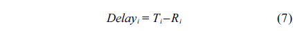
For other non-split tasks, the delay is considered as in Formula (7). As mentioned earlier, scheduling in the ready queue is based on the rate monotonic algorithm, so the worst response time of task
τi is feasible under rate monotonic → Ri ≤ Ti Delayi = Ti –Ri RiSS–DRM = Ti –Ri+Ri
The worst response time of task
Therefore, it is proven that all non-split tasks, which are feasible under the rate monotonic algorithm, are feasible under SS-DRM as well. So, the response time analysis can be used for admission control of SS-DRM.
In SS-DRM, based on the delayed rate monotonic algorithm, a non-split task which is in the delay queue can run next if the ready queue is empty. According to Formula (8), the delay of a split-task is equal to the total worst-case execution time of prior subtasks. It means that with the delay of subtasks, we express the concept of release time used in another study [4]. Now, a split-task in SS-DRM can run only if its delay is completely finished and it has entered the ready queue.
This is done to synchronize subtasks of a split-task. In this work, the same behavior for a split-task as it is regarded in RM-TS is considered. More details on the feasibility of the split-tasks are presented in a previous study [4]. In this work, to use the advantages of the delayed rate monotonic algorithm, such as its resilience against possible overload, the allocation method of RMTS is adapted to this algorithm.
>
A. Changing Assigning Method
To improve the processor utilization under the SS-DRM algorithm, we express two improvements. First, Theorem 1 is stated.
THEOREM 1.
First, a system composed of two non-split tasks. Suppose two non-split tasks τ1(C1, T1) and τ2(C2, T2) are assigned to a processor, T2 > T1 and U1 + U2 ≤ 1. According to Relation (7), the delay of task τ1 under SSDRM is equal to T1 – R1. Considering Formula (4), the worst response time of the highest priority task is equal to its worst-case execution time, so the delay of task τ1 is equal to T1 – C1, and this system is scheduled safely under SS-DRM. The second type of system is composed of two tasks and includes a non-split task τ1 (C1, T1) and a split-task in which is the last subtask of split-task τ2.
To illustrate this system, suppose
We know that and in real-time systems the worst-case execution time of a task is at most equal to its period. Now, we have:
Therefore, the delay of subtask in processor
In Theorem 1, it is expressed that because of the third type of system, the task
● The third type of a system composed of two tasks is a system which consists of a non-split task
The delay of this subtask is equal to zero and it directly enters the ready queue. The fact that their total utilization is less than one does not guarantee the feasibility of these tasks under SS-DRM. Therefore, this state is separated in Theorem 1.
Now, we use Theorem 1 to express two improvements in allocation method of SS-DRM. These improvements make SS-DRM achieve higher processor utilization than RM-TS. The first improvement is a new pre-assignment function, and the second improvement is a new splitting function. In the new pre-assignment function of SSDRM, we try to fully utilize the existing processors by assigning two tasks with total utilization in a specific bounds to each processor.
For each task
Condition (9) determines the specific bounds of processor utilization of pre-assign processors. The lower bound, δ, is
First, we try to find some groups of two tasks, each with total utilization satisfying Condition (9). Then, each group is assigned to a single processor. These processors are removed from the queue of processors, and hence, no other task or subtask is assigned to these processors.
After the pre-assignment function, it is time for remaining tasks. These tasks are assigned to the remaining processors, just like in the assignment method used in RMTS.
From Algorithm 2, it is easy to derive the following property.
LEMMA 4.
Therefore, Theorem 2 can be stated.
THEOREM 2.
Therefore, using this pre-assignment function, some processors exist in which the processor utilization is raised up to 100%. Another advantage of the new preassignment function is the number of created subtasks. The number of created subtasks is at most m – 1 [4]. Based on the new pre-assignment function, after assigning two tasks to one processor, no other task or subtask is assigned to this processor. Therefore, the number of created subtasks in SS-DRM is smaller than that of RM-TS, and due to the number of created subtasks, the additional overhead of the system is reduced.
The second improvement proposed for the allocation method of SS-DRM in order to improve the processor utilization is a new task splitting function. This function uses the second type of system composed of two tasks, which is expressed in Theorem 1. Two assumptions exist in our splitting function.
Assumption 1. The current task in front of the queue of un-assigned tasks is a subtask, i.e., ,
Assumption 2. The host processor includes only one non-split task
If these two assumptions hold, then tasks
Now, in the new splitting function of SS-DRM, and such a situation, if the total utilization of two tasks,
Algorithm 3 demonstrates the pseudo-code of the new splitting function of SS-DRM. Three parameters are inputs of this algorithm: first, the current task; second, a task set Γ' which illustrates all assigned tasks to the host processor; and third, the delay of the current task.
As mentioned earlier, the delay of non-split tasks is calculated by Formula (7). This delay is calculated in the scheduling phase when all tasks are clearly assigned to the processors. Therefore, in the partitioning phase, the delay of non-split tasks is assumed to be zero (line 2 of Algorithm 1). On the other hand, for split-tasks, the delay is calculated in the partitioning phase, so their delay is not equal to zero (line 29 of Algorithm 1).
The longest value for the worst-case execution time of the current task by which all tasks in Γ' are feasible is the output of this algorithm. Based on this function, in some processors, SS-DRM can raise the processor utilization to 100%.
In line 6 of Algorithm 3, we check two assumptions. First, only one task exists in the host processor;
In the following, we illustrate an example to show the performance of our splitting function.
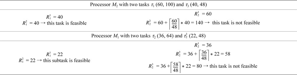
EXAMPLE 2. There are two processors,
[Table 2.] Period and worst-case execution time of tasks
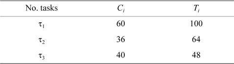
Period and worst-case execution time of tasks
According to row two of Table 3, the current task,
[Table 3.] Check feasibility of tasks using response time analysis

Check feasibility of tasks using response time analysis
For finding a suitable value for , the splitting function is called. This subtask is the first subtask of split-task
Therefore, it should be split into two subtasks ( ,
The output of the splitting function of SS-DRM is equal to 21. It means the value of the worst-case execution time of is obtained as 21, and the processor utilization of
If we use a simple binary search which has to be used for RM-TS, the worst-case execution time of reduces to 14. In this case, the processor utilization of
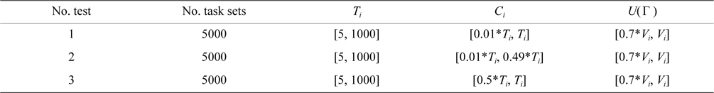
In this section, we investigate the performance of SSDRM compared with three prior works. In our evaluations, three different kinds of task sets are randomly generated. The distribution of our random function is uniform. The details of each task set are shown in Table 4.
[Table 4.] Features of each test

Features of each test
The total utilization of each task set,
[
We assume that:
where
For instance, when
We define another parameter called the average processor utilization to evaluate each algorithm. This parameter is calculated by Formula (10).
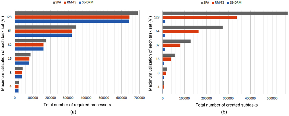
First, we compare SS-DRM with SPA [7] and RM-TS [4]. In the first row of Table 4, the features of generated task sets are illustrated. For instance, the utilization of each task is randomly selected from 0.01 to 1 and consists of both light tasks and heavy tasks.
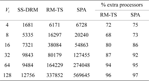
The total number of required processors in the system are demonstrated in Fig. 1(a) and Table 5 through the three aforementioned algorithms. Fig. 1(b) and Table 6 show the total number of subtasks which are created by these three algorithms. As shown in Fig. 1(a) and Table 5, by increasing the value of
[Table 5.] Total number of required processors
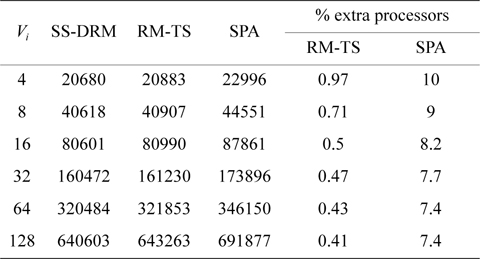
Total number of required processors
[Table 6.] Total number of created subtasks

Total number of created subtasks
Considering Fig. 1(b) and Table 6, the difference of the total number of created subtasks under SS-DRM compared with RM-TS or SPA is remarkable. As mentioned earlier, the overhead of task splitting is the same as previous works. Therefore, by creating a lower number of subtasks, the overhead of task splitting is reduced in comparison to RM-TS and SPA. This difference occurs because of the pre-assignment function of SS-DRM. As
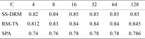
Table 7 illustrates the average processor utilization of three algorithms. It can be observed that SS-DRM significantly achieves better average processor utilization in comparison to SPA and RM-TS. The average processor utilization of SS-DRM is about 0.58% and 10% more than RM-TS and SPA, respectively.
[Table 7.] Average processor utilization

Average processor utilization
The average number of callings of our new splitting function in all simulations is about 1.1% of the total number of processors. It means that the processor utilization of 1.1% of the processors is almost equal to one. These processors have two tasks: a non-split task and a splittask. The split-task is not the first part of the task which is split. Their safety is assured by Theorem 1.
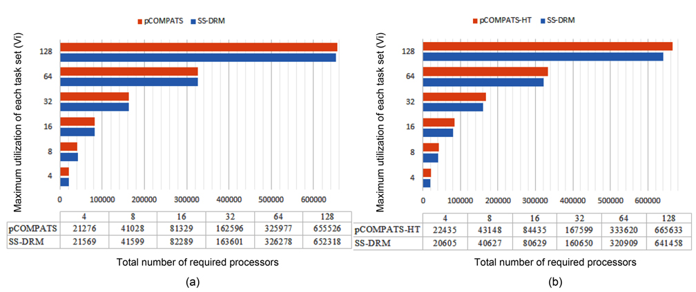
The second row in Table 4 shows tasks with random utilization between 0.01 and 0.49 in order for SS-DRM to be comparable with pCOMPATS [6]. As mentioned earlier, tasks in pCOMPATS are divided into two groups: light and heavy. For each group, a separate approach is proposed. A first-fit method is used for allocating light tasks (tasks with utilization lower than 0.5).
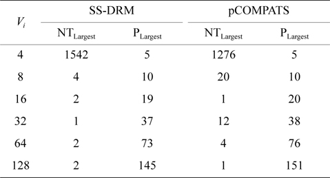
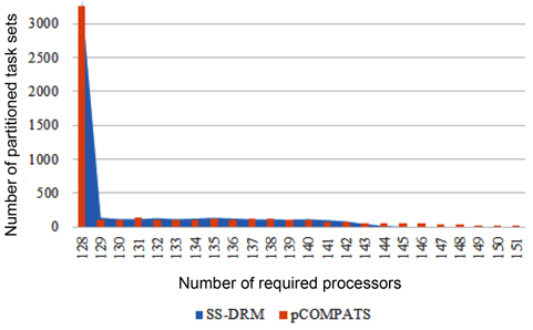
In this approach, the lowest priority task is split. pCOMPATS uses R-Bound for the schedule-ability test to cluster compatible tasks together. Table 8 shows the average processor utilization, and Fig. 2(a) shows the total number of required processors. As shown in Fig. 2(a), the performance of pCOMPATS is a little better than SSDRM. Since the utilization of each task is less than 0.5, it is hard to find a system composed of two tasks in which the total utilization of a system is near one. Therefore, the pre-assignment function of SS-DRM is not used much. But the largest number of required processors in pCOMPATS is more than the largest number of required processors in SS-DRM. Details of the largest number of required processors for each approach are shown in Table 9.
[Table 8.] Average processor utilization
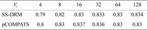
Average processor utilization
[Table 9.] The largest number of required processors

The largest number of required processors
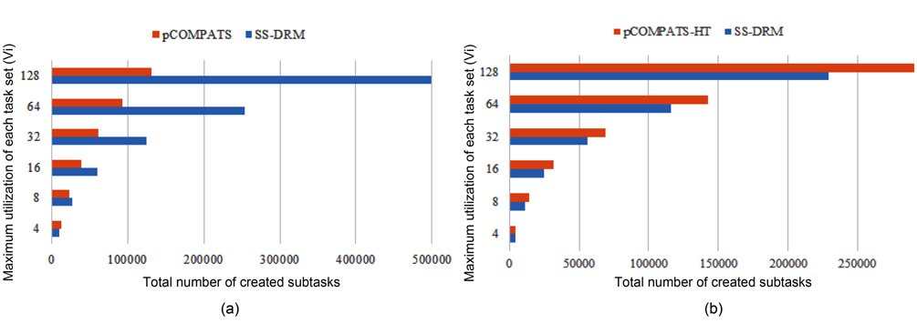
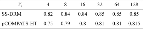
The total number of created subtasks by two approaches is shown in Fig. 4(a). Considering Fig. 4(a), the total number of created subtasks by SS-DRM is more than pCOMPATS, since pCOMPATS uses the first-fit method to allocate compatible tasks to one processor. The disability of pCOMPATS to partition tasks with utilization larger than 0.5 is the main challenge of this approach. The third group of generated task sets is used to compare SS-DRM with pCOMPATS-HT. In [6], pCOMPATS-HT is proposed to assign heavy tasks (tasks with
In pCOMPATS-HT, tasks are sorted in descending order of their periods. First, one task is assigned to each empty processor. If no empty processor is found, and the current processor is not full, then the current task is split into two subtasks. According to the sorting method, the highest priority task is split. Fig. 2(b) shows the total number of required processors under SS-DRM and pCOMPATS- HT.
As shown in Fig. 2(b), the difference of the total number of required processors between two approaches is remarkable. The total number of created subtasks is more proof which indicates the superiority of SS-DRM compared to pCOMPATS-HT. The total number of created subtasks by two approaches is demonstrated in Fig. 4(b).
According to the utilization of each task, most processors have two tasks. The total utilization of two tasks is at least equal to one. Therefore, the pre-assignment function of SS-DRM is not useful here. On the other hand, the splitting function of SS-DRM can be used to split a task in order to fully utilize processors. For instance, when
[Table 10.] Average processor utilization

Average processor utilization
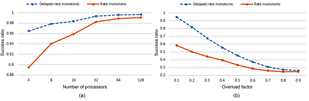
For evaluation of the delayed rate monotonic algorithm against overload, we randomly generated 1000 task sets for each test. These task sets are generated so that they can be completely assigned to the processors. The allocation method of RM-TS is used for assigning tasks. For producing overload, a task is randomly selected, and its execution time is somewhat increased. Then, the executions of these task sets are simulated under both the rate monotonic algorithm and the delayed rate monotonic algorithm.
For the first evaluation, a task is randomly selected, and its execution time is enlarged so that its overload factor is increased by 0.1, 0.2, and 0.3 for three different tests. At the end, the success ratio average of these tests is computed for the corresponding number of processors. Fig. 5(a) shows the result of this evaluation. As shown in Fig. 5(a), the success ratio of two algorithms when the number of processors is high becomes closer. This happened because the number of processors which are not overloaded is increased as well.
In the second evaluation, for each processor, a task is randomly selected, and the overload factor is added to its worst-case execution time. Fig. 5(b) shows the result of this evaluation for 32 processors. The success ratio of two algorithms converges together with increasing overload factor, because the number of processors with utilization larger than one is increased as well.
In this paper, a new scheduling algorithm called SSDRM was proposed by combining the delayed rate monotonic algorithm with a semi-partitioned technique. SS-DRM can safely schedule any task set which is feasible under the rate monotonic algorithm.
Our proposed approach can increase the processor utilization beyond the well-known L&L bound. SS-DRM can also be more resilient against possible overload compared with the rate monotonic algorithm. Further, it achieves the same utilization. Then, we expressed two improvements to achieve higher processor utilization in some special cases under the SS-DRM algorithm. In our future works, further improvements will be sought to change the allocation method of SS-DRM to improve the processor utilization.