Recently, the use of UAVs has been expanded in both military applications and civil operations [1-3]. When a UAV performs a mission such as surveillance, it is more advantageous to utilize multiple UAVs rather than a single UAV [4]. The task can be performed in a group of multiple UAVs, which can deal with the failure due to the loss of a UAV from an enemy attack or hardware/software fault. In addition, the range of operations can be extended.
To make UAVs move in formation, it is required that a proper method for formation flight which has physical reasonability be proposed and the proposed method should have a definite performance in terms of exactness of formation configuration. Formation flight of UAVs can be accomplished by several methods, which include the leader-follower approach, virtual structure approach, behavioral approach, and so on [5]. Among those methods, the virtual structure approach is more physically comprehensible compared to the others and can easily construct a formation shape.
To make UAVs cope with collision threats instantly, it is required that a proper method for collision avoidance which is simple and effective be proposed. Collision avoidance for a UAV can be accomplished by various methods such as the potential field method, geometric approach, grid based method, generic algorithm, and so on [6-7]. Among those methods, the potential field method is quite attractive in that it is easy to understand intuitively and its potential function, which is used to generate commands, can be made freely according to specific objectives. The geometric approach is also easy to understand and can be used simply.
For the operation of multiple UAVs, it is important to consider both formation flight and collision avoidance. In Ref. [8], formation flight and collision avoidance were considered separately and changed the modes according to the flight situation. In Refs. [9] and [10], formation flight and collision avoidance were considered at the same time with weighted sum of certain functions. Those works [8-10] lack effort for considering formation flight and collision avoidance simultaneously. Especially, in Refs. [9] and [10], weighting values used in the consideration were defined as constants, which may lead to inefficiency in coping with unexpected collision threats. Also, there is no convincing explanation for the reason why the weighting values were chosen. Thus, it is strongly required to develop the proper methods for formation flight and collision avoidance regarding multiple UAVs and connect those methods with an appropriate weighting value. The value should be defined reasonably and vary with the situation continuously.
In this thesis, a physically appropriate method for formation flight based on the decentralized virtual structure approach and a simple method for collision avoidance using the geometric approach are proposed separately. Both methods are connected by a concept of elastic weighting factor that is inspired by the behavior of the material which exists in nature. Using the concept, UAVs can deal with the collision threats including the other UAVs in formation and unknown obstacles during flight simultaneously.
This paper is organized as follows. Section 2 proposes the formation flight method based on the virtual structure approach. The stability of the proposed method is analyzed using the Lyapunov Stability Theorem. Section 3 gives the collision avoidance method based on the geometric approach, and stability analysis on the proposed method is also performed using the Lyapunov Stability Theorem. Section 4 introduces the concept of elastic weighting factor for the integration of heading commands. Section 5 provides numerical simulation results in which a performance of the proposed method is verified. Finally, section 6 is devoted to the summary of the main results and the future work.
A formation flight method proposed in this section is based on the following assumptions.
Assumption 2.1. There is a certain range in which UAVs can communicate.
Assumption 2.2. UAVs can obtain information which includes the position and velocity of other UAVs within the range.
2.1 Coordinate System and Kinematics for Guidance
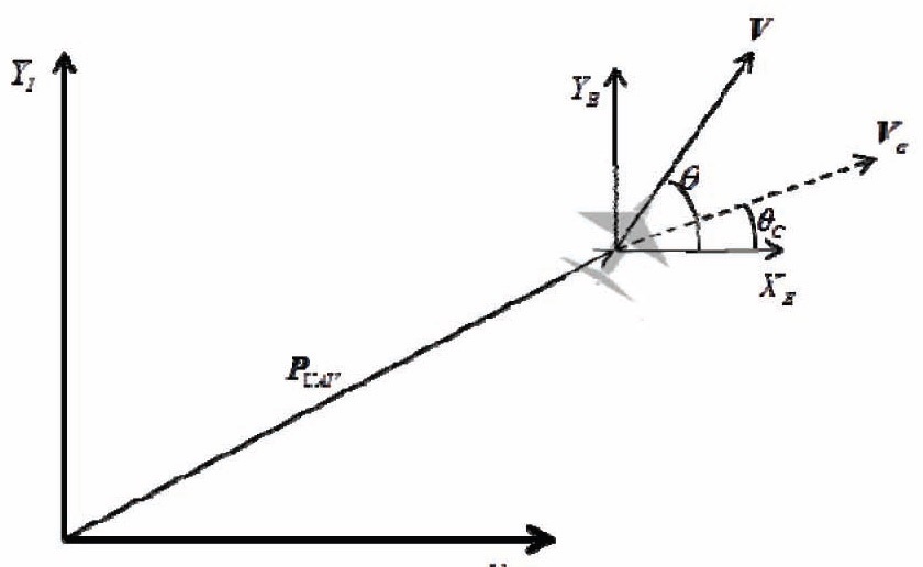
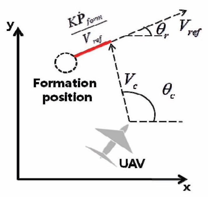
All geometric information used in this study is based on a two dimensional cartesian coordinate system. Two coordinate frames are considered; the inertial coordinate frame and body fixed coordinate frame. Position information is expressed in terms of the inertial coordinate frame. Heading angle and speed of UAVs are represented in terms of body fixed frame. Let us consider a position of a UAV expressed as follows:

Note from Eq. (1) that the position is expressed in the inertial coordinate frame only, and therefore subscript I will be omitted in the remaining sections for simplicity. To visualize the coordinate system as shown in Fig. 1, let us consider the flight situation of a single UAV with the following velocity command:

where
as the current position vector of UAV, and


where

2.2 Heading Command and Speed Command
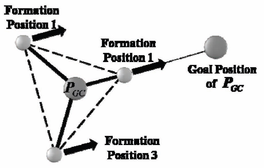
Formation flight is performed in a way that each UAV pursues its formation position that is defined through the virtual structure. To construct the virtual structure, let us define the geometric center of UAVs as follows [11]:
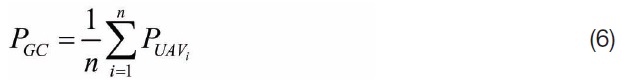
where

and
denote the position vector of the geometric center and a


where
Using the look-ahead factor
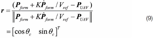
Where

From Eq. (9), the heading command can be expressed as
follows.
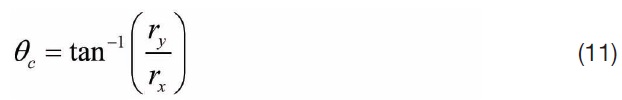
where (
2.3 Stability Analysis and Speed command
2.3.1 Stability Analysis
To guarantee that a position of a UAV converges to the formation position with the heading command defined in Eq. (11), a stability analysis using the Lyapunov stability theorem is performed and the detailed procedure is explained in Ref. [12].
From Ref. [12], a condition for the time derivative of the Lyapunov candidate function to be negative can be obtained as follows.
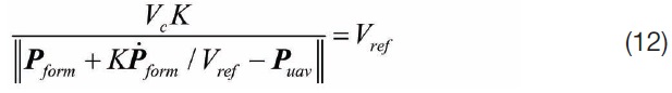
Eq. (12) is an important condition for deciding the lookahead factor and
Note from Ref. [12] that the time derivative of the Lyapunov candidate function has a negative value except the case when the position of a UAV and the formation position are coincident. This means that the value of the Lyapunov candidate function is decreasing and converges to zero asymptotically. As the Lyapunov candidate function is defined as a distance from the UAV position to formation position, it means that the distance is decreasing and become zero eventually.
2.3.2 Look-Ahead Factor and Speed Command
To make the heading command appropriate for the formation flight and generate a proper speed command, Eq. (12) should be considered. Two unknown variables,

Using Eq. (12), the constraint condition on the speed command can be expressed as follows:
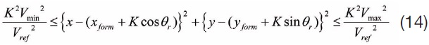
With the properly pre-defined constant value of
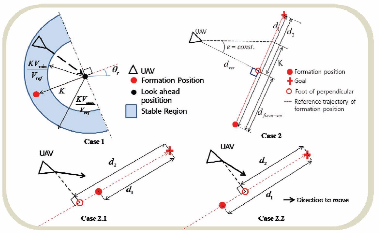
Case 1. For the case that Eq. (14) is satisfied. : A UAV is in the stable region where the convergence to the formation position is assured.
Case 2. For the case that Eq. (14) is not satisfied. : A UAV is outside the stable region.
The descriptions of each case are shown well in Fig. 4.
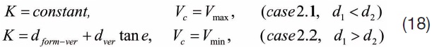
Case 2 can be categorized again into two sub-cases.
Case. 2.1 Pursuing case

: As a projected position of a UAV is farther from the goal point than the formation position, the UAV needs to pursue the formation position.
Case. 2.2 Pursued case

: As a projected position of a UAV is closer from the goal point than the formation position, the UAV needs to be pursued by the formation position.
In Fig. 4,
Variables
Case 1:
Case 2:
where
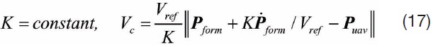
With Eq. (9), Eq. (17) and Eq. (18), guidance commands for formation flight including the heading command and the speed command are generated. As case 2 is always turned into case 1 eventually, which means that the UAV moves towards the stable region and enters the region in the end, the convergence of the UAV to the formation position is assured in all flight situations.
The collision avoidance method proposed in this section is based on the following assumptions.
Assumption 3.1. Assumptions of section 2 are still valid.
Assumption 3.2. All obstacles are static.
Assumption 3.3. There exists a ‘safety range’ and ‘sensing range’ between the UAV and static obstacle.
Assumption 3.4. There exists a ‘safety range’ and ‘sensing range’ between the UAV and other UAVs.
The safety range means a minimum distance which a UAV should have for the collision avoidance of the threat. Also, the sensing range means a distance in which the UAV recognizes a threat.
The proposed method in this section deals with the procedures of generating the command for the collision avoidance of a single threat. And the method will be extended to multiple threats with a proper weighting value in section 4.
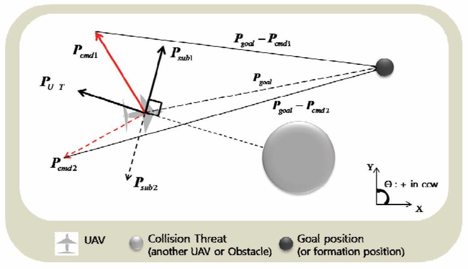
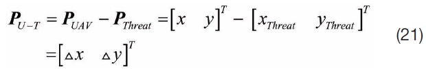
The direction of the relative position vector can be used to increase a distance between the UAV and the threat. Another vector is also considered by defining sub-vectors which are perpendicular to the relative position vector as shown in Fig. 5. In Fig. 5,
The heading command can be generated by using vectors which are defined in Fig. 4 as follows:
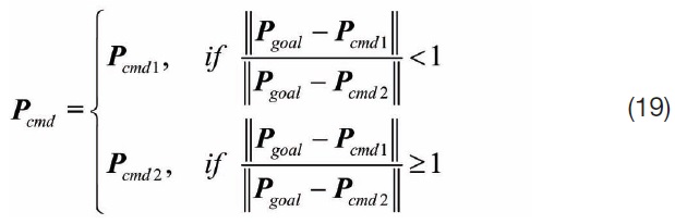
In Eq. (19),

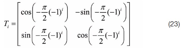
In Eq. (20), i denotes the mode of the sub-vector, and decides the direction, i.e., +90° for

In Eq. (22),
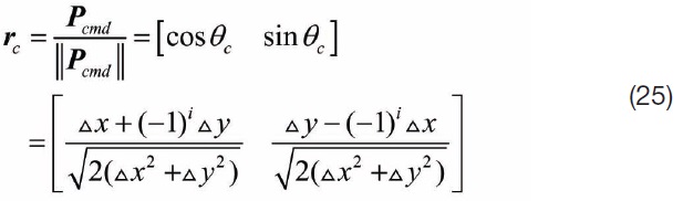
Using Eq. (21) and Eq. (23),

Using Eq. (27), the heading vector which the UAV should follow can be written as:
Finally, the heading command can be generated by using Eq. (25) as:
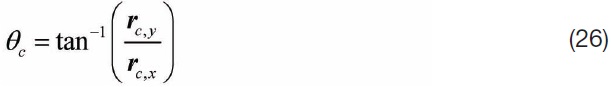
where
A stability analysis for the proposed heading commands is performed using the Lyapunov stability theorem. The analysis assures that the UAV always moves in the direction away from the threat and avoids the collision threat surely whether it is another UAV or a static obstacle. Ref. [12] contains a detailed procedure of the analysis.
4. Combined Guidance Law for Formation Flight and Collision Avoidance
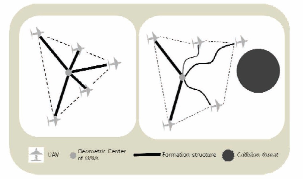
In general, the virtual structure approach deals with a fixed shape of formation. In other words, the structure is notionally treated as a rigid body. In this type of structure, the group of UAVs cannot react effectively to unexpected situations including a collision. This problem can be solved by giving the elastic property to the structure using the Elastic Weighting Factor (EWF). A main idea of the EWF is to provide an elastic property to the virtual structure as shown in Fig. 6. Using this concept, the structure of the formation is deformable during flight, and therefore UAVs can easily cope with the collision threat.
Among many materials in the real world, SMP (Shape Memory Polymer) has properties of the deformable formation structure. The SMP has the shape memory effect and the elastic behavior which can be applied to the structure. Depending on the external stimulus like temperature, the shape or length of the SMP is variable. When the external stimulus returns to the certain condition, the SMP recovers its permanent or original shape. Using this property, the formation structure can be deformed considering an effect from the collision threat and return to its original state. The formation structure can have a soft phase or a state like a rubber band for the collision avoidance as well as a hard phase or a rigid state for maintaining the formation structure.
When adapting the SMP to the formation structure, the elastic modulus of the SMP corresponds to the material property of the structure and the temperature which is an external stimulus corresponds to a distance from a UAV to the collision threat. In other words, the structure’s property varies according to an interaction between the UAV and all the threats within the sensing range in which the UAV recognizes the risk of collision.
4.2. Shape Memory Polymer Modeling
In this section, the model of SMP is represented. The elastic weighting factor,
Definition 4.1 (Elastic Weighting Factor,
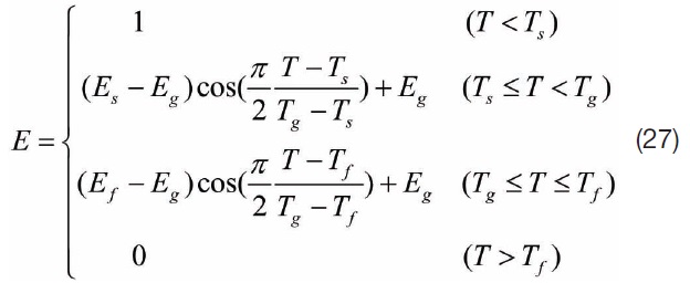
where
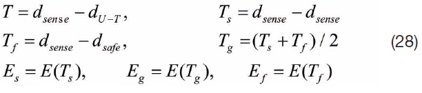
Note that subscript s represents the sensing range where a transition from a rigid to elastic state starts, and subscript
4.3. Combination of Heading Commands
To adapt
Definition 4.2 (E for
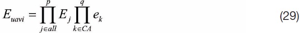
where the value of
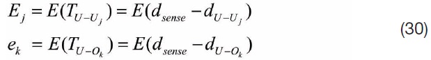
In Eq. (30),
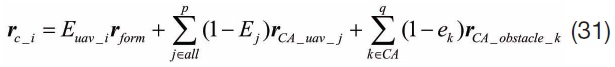
In Eq. (31),
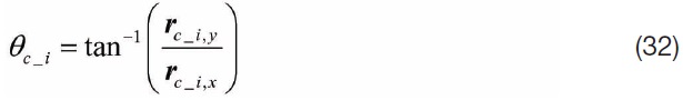
where
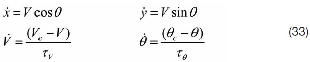
The two-dimensional point mass model of UAV is used in the simulations. To consider the time delay of UAV dynamics and autopilot, heading angle
[Table 1.] Parameters and initial values

Parameters and initial values
where
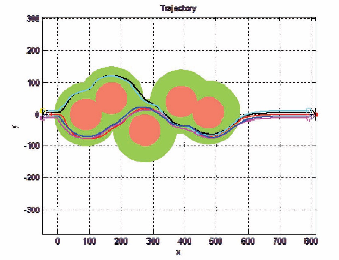
To check the performance of the proposed method, a situation of collision avoidance during the formation flight is simulated. That is, UAVs encounter unknown static obstacles during the formation flight. It is required for UAVs to avoid the collision threats by deforming the formation. After the avoidance is finished, UAVs have to recover their formation.
The parameters and initial conditions of the simulation environment are summarized in Table 1.
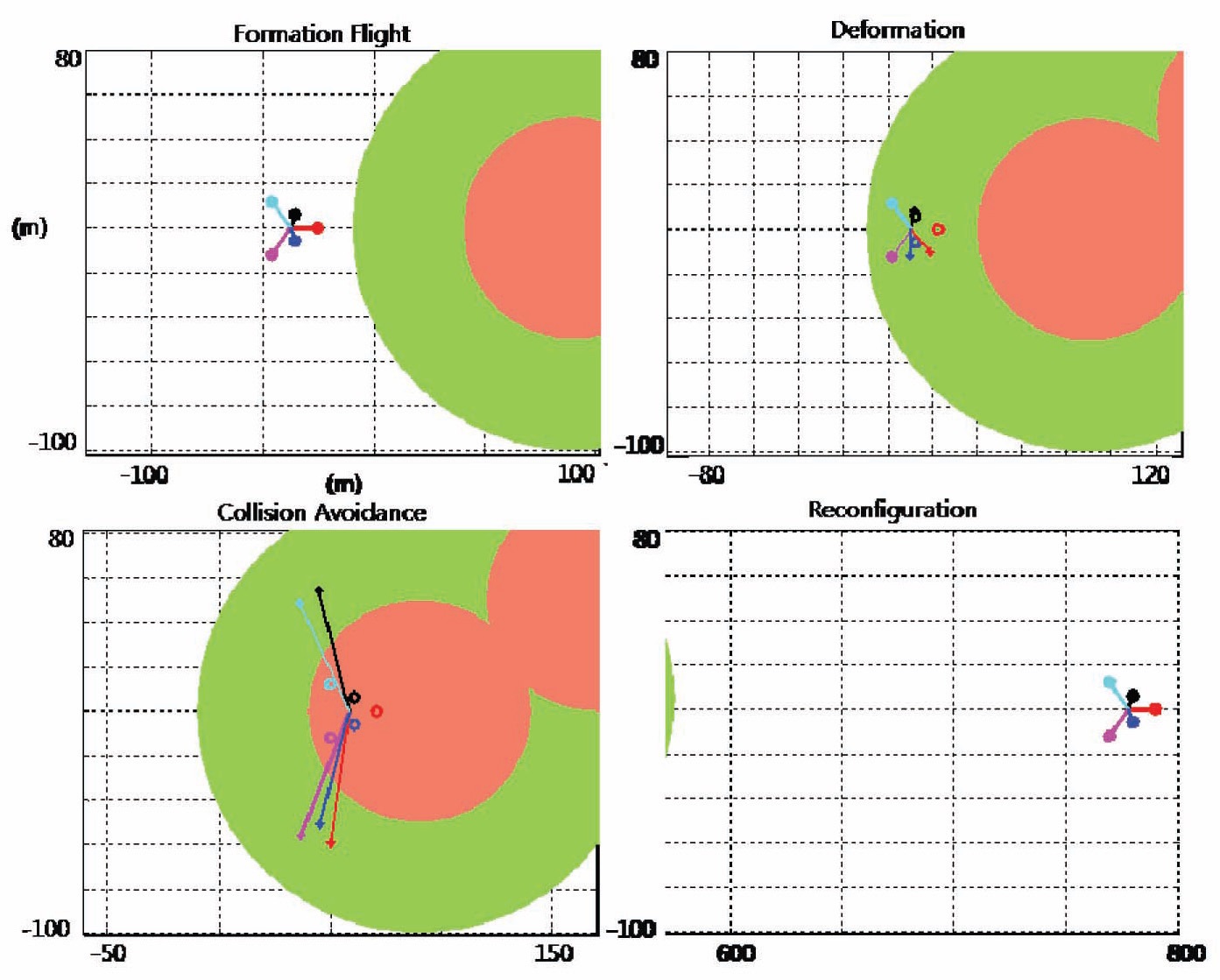
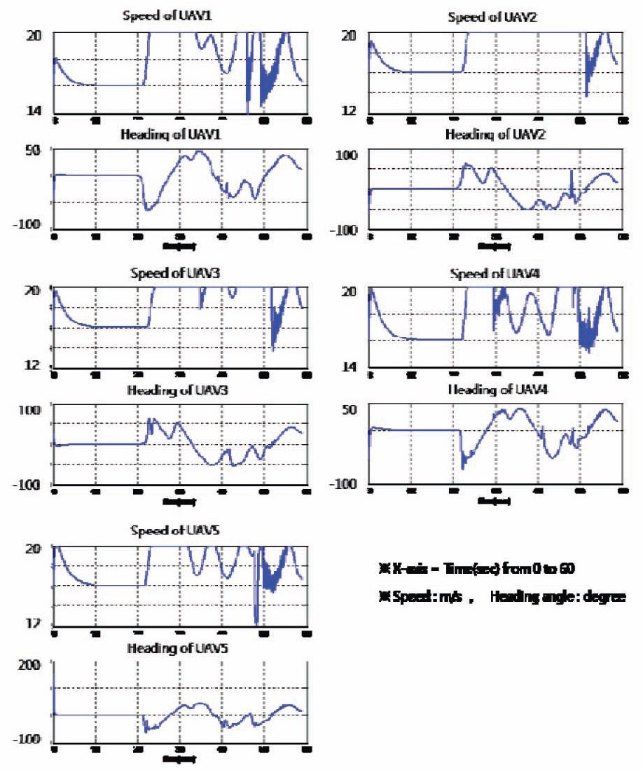
Figure 7 shows the trajectories of each UAV. It can be seen that the collision avoidance during the formation flight is performed successfully. The elastic behavior of the formation structure is shown in Fig. 8. When UAVs recognize the collision threats, the formation structure varies elastically so that UAVs can avoid the threats effectively, and then recover its original formation after the avoidance. In Fig. 9, fluctuations are observed in the speed of UAVs,
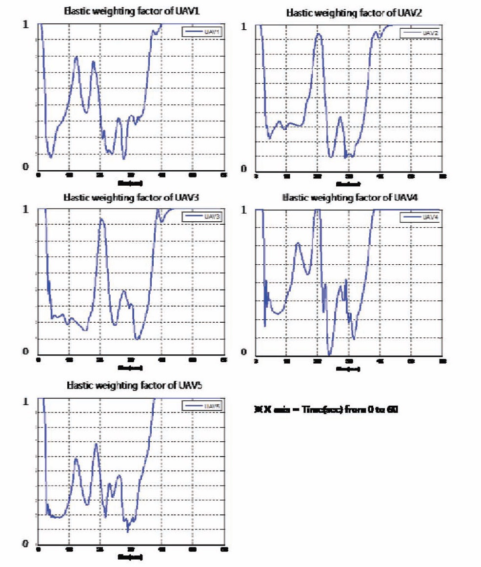
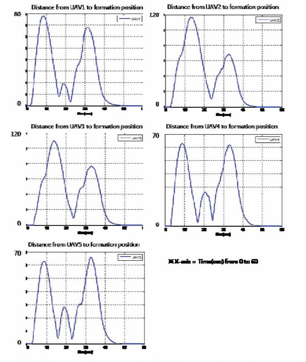
because UAVs repeatedly come in and out of the region where the stability is assured as the collision avoidance and the formation flight are considered simultaneously. Heading angles vary quite smoothly as shown in Fig. 9. In Fig. 10, it also can be seen that the concept of elastic weighting factor is used well in the presence of unknown obstacles. In addition, elastic weighting factors change continuously considering both other UAVs and unknown obstacles. In Fig. 11, all UAVs converge to their formation position after the avoidance.
To see the performance of collision avoidance with threats
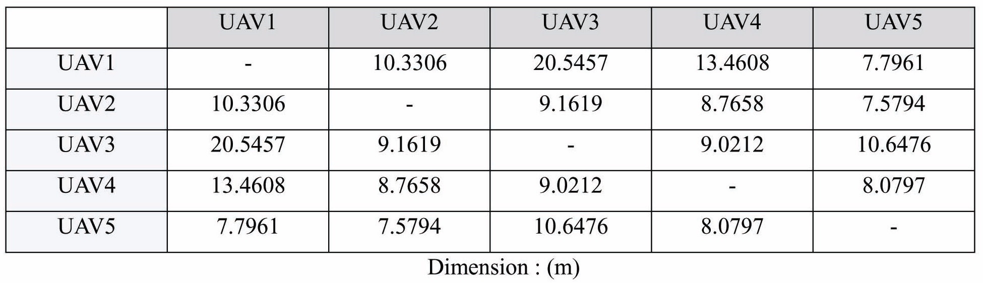
[Table 2.] The minimum distances among all UAVs

The minimum distances among all UAVs
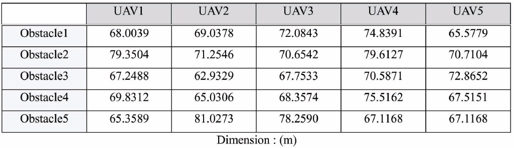
including other UAVs and obstacles, the minimum distances among all UAVs are summarized in Table 2 and minimum distances from each UAV to the unknown obstacles are summarized in Table 3. As it can be seen in Tables 2 and 3, all UAVs maintain their distance farther than the safety range from other UAVs and obstacles. Thus, it can be said that collision avoidance during the formation flight is well performed.
Guidance laws for decentralized formation flight and collision avoidance are proposed. The stability of the each guidance law is proved using the Lyapunov Stability Theorem. By introducing the concept of elastic weighting factor, heading angle commands of formation flight and collision avoidance are integrated. The integrated guidance law makes UAVs perform formation flight and collision avoidance simultaneously. It is shown that UAVs can cope with the collision threats including other UAVs in the formation and unknown obstacles. The guidance command
for UAVs can be generated by a simple calculation at every moment, and therefore the proposed method can be utilized for real time applications.
[Table 3.] The minimum distances from each UAV to unknown obstacles

The minimum distances from each UAV to unknown obstacles