Recently, many studies on autonomous flights of Unmanned Aerial Vehicles (UAVs) have been performed, since UAVs have been used to accomplish various missions. In particular, target observation mission has been widely studied, because it has very important applications, such as aerial reconnaissance and surveillance. Multiple small UAVs may substitute for a large UAV, for performing complicated missions, due to their low cost and easy operation, and therefore various guidance laws for multiple UAVs have been developed [1-8].
A vector field approach has been studied for standoff tracking missions of multiple UAVs [1-6]. A Lyapunov vector field was used to calculate the desired velocity and heading rate of UAVs, for performing coordinate standoff tracking of a stationary or moving target [1-4]. Chen et al. modified the Lyapunov vector field, by combining a tangent vector field, to find a short path for a UAV tracking a ground target [5]. Lawrence et al. extended the Lyapunov vector field guidance for path and waypoint passing, by switching circular loiter vector fields [6]. The Lyapunov vector field guidance law guarantees global stability, by showing limit cycle behavior about circular loiter patterns. However, due to the limit cycle behavior, it is difficult to implement it in missions in complexly constrained environments.
Distance error dynamics were also utilized, to design a guidance law for performing stationary target observation [7,8]. Distance error and Line-of-Sight (LOS) information were used to guide a UAV to the observation circle, utilizing the characteristics of distance error dynamics. Distance error dynamics-based guidance law has a simple structure, but it does not guarantee the satisfaction of various constraints on time or angle.
This paper deals with a waypoint constraint problem on the observation circle. Time and angle constraints to approach the desired circle path could become important issues for multiple UAVs operation, to avoid them colliding with each other, and to perform the mission effectively. While the time and angle constraints problem has not been treated much in UAV systems, similar problems have been widely studied in missile systems [9-12]. Impact time and impact angle constraints in missile systems, which have the same meaning of approach time and incidence angle, are very important in attacking a target. For this reason, a nonlinear guidance law used in missile systems is considered, to solve the waypoint constraint problem in this study.
Pseudo pursuit guidance law and distance error dynamicsbased guidance law are utilized, to perform the stationary target observation of multiple UAVs, with waypoint incidence angle constraint. The whole guidance logic consists of two steps: the waypoint approach step, with specified incidence angle; and the loitering step, around the stationary target. In the first step, UAVs fly to the waypoint, using pseudo pursuit guidance law. After passing the waypoint, UAVs turn around the target, using the distance error dynamics-based guidance law, which is the second step.
The purpose of the paper is to propose a nonlinear guidance scheme, by implementing two nonlinear guidance laws that are easy to understand and simple to implement. Therefore, the proposed guidance scheme is used to satisfy the waypoint incidence angle constraint, and to perform the stationary target observation mission.
This paper is organized as follows. Section 2 provides the waypoint determination, using the geometric relation among UAVs and the stationary target. Pseudo pursuit guidance law considering the desired heading angle and distance error dynamics-based guidance law is also described. Section 3 shows numerical simulations for verifying the performance of the proposed nonlinear guidance scheme. Finally, the conclusion is given in Section 4.
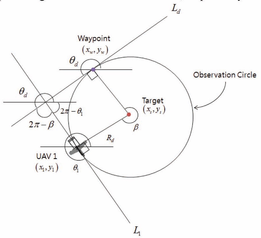
Waypoint constraint could be given, to complete a given mission effectively and successfully. In this study, the following assumptions are considered. First, the velocity of the leader UAV is constant, but the velocity of the follower UAV could be changed, to maintain the distance from another UAV. Second, in the beginning, all UAVs fly to their initial waypoint. However, when the leader UAV passes its waypoint, and starts to loiter around the stationary target, the follower UAVs’ desired waypoints are changed, according to the position of the leader UAV turning around the target. Third, follower UAVs have the information of the leader UAV position and turning direction. The first and second assumptions are the mission considered in this study, and the third one is necessary for UAVs to avoid colliding with each other. Figure 1 describes the waypoint determination process of the follower UAVs, while the leader UAV turns around the stationary target.
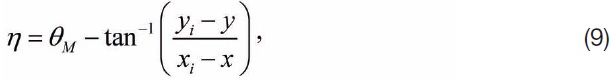
In Fig. 1, (
Definition 1. The directions of UAV LOS angle and UAV heading angle are positive counterclockwise (CCW) from the x-axis. The direction of the phase angle is positive CCW from the radius of the loitering UAV.
From the geometry in Fig. 1, the desired heading angle of the approaching UAV can be obtained as

where,
For the operation of multiple UAVs, the turning direction of each UAV should correspond with the turning direction of other UAVs, to avoid colliding with each other. To determine the waypoint that the follower UAV approaches on the observation circle, the desired LOS angle should be obtained.
Proposition 1. For a CW turn case, the desired LOS angle is determined by subtracting
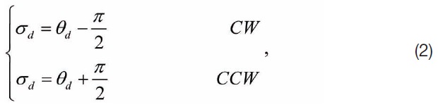
where,
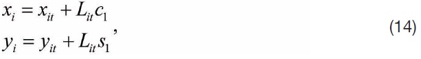
Then, the position of the approaching waypoint on the observation circle is calculated as
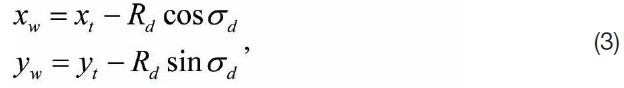
The approaching waypoint will move along the observation circle whose radius is
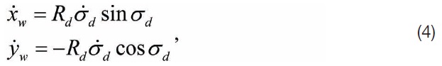
Let us substitute eqs.(2) and (3) to eq.(4).
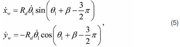
Finally, the movement rate of the waypoint can be represented as
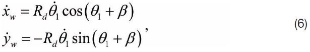
As the approaching waypoint of the follower UAV moves,
the follower UAV should accelerate or decelerate, to reduce or increase the phase angle between the leader UAV and the follower UAV, and finally maintain the desired phase angle difference. Therefore, the following velocity command is required for the follower UAV [1,2].

where,
2.2 Pseudo Pursuit Guidance Law
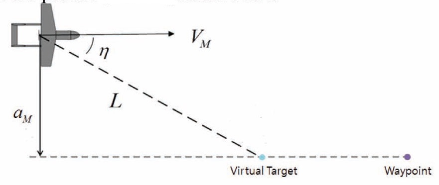
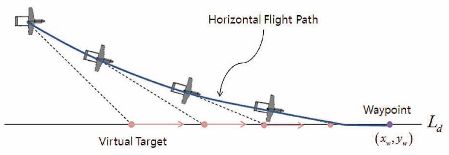
Pursuit guidance is one of the widely used guidance laws for a missile system. Pseudo pursuit guidance law was introduced for automatic landing of a fixed wing UAV to a recovery net [13]. While the pure pursuit guidance law leads a UAV to a true target directly, the pseudo pursuit guidance law generates a guidance command for the vehicle to a virtual target. As the virtual target moves to the true target, the UAV finally arrives at the true target. Figure 3 explains the concept of the pseudo pursuit guidance law.
In Fig. 3,
To satisfy the waypoint constraint, the virtual target is sequentially generated on the tangent line,
Figure 4 shows the flight path of the UAV, and the movement of the virtual target on the tangent line, by using the pseudo pursuit guidance law.
Let us assume that the flight direction of the UAV is the same as the velocity vector direction of the UAV. In other words, the heading of a UAV aligns with its velocity vector. Then, the angle between the velocity vector and the virtual target,
where,

represents the direction vector of the virtual target movement on the tangent line.
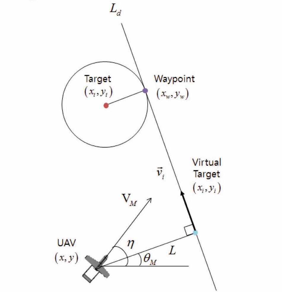
Now, let us consider another important issue, that is, how to determine the virtual target. Note that the imaginary target is located on the tangent line, and it moves to the waypoint. Therefore, the following equation can be obtained from the geometric relation between the virtual target and the true waypoint.

Let us assume that the direction vector of the virtual target is perpendicular to the line between the UAV and the virtual target. Then, the following equation can be obtained.

Let us redefine the temporary virtual target, satisfying the above assumption, and the geometric relation between the true waypoint and the virtual target. Then, the position of the temporary virtual target can be calculated as
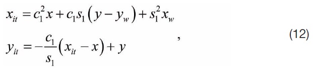
where,
If the desired heading angle is set as 0 or 180 degrees, then the position of the temporary virtual target should be chosen as
To rapidly guide the UAV, the virtual target should be located in front of the temporary virtual target, considering the direction of the movement. Figure 6 shows the geometric relation of the true waypoint, the virtual target, and the temporary virtual target.
In Fig. 6,
2.3 Distance Error Dynamics-Based Guidance Law
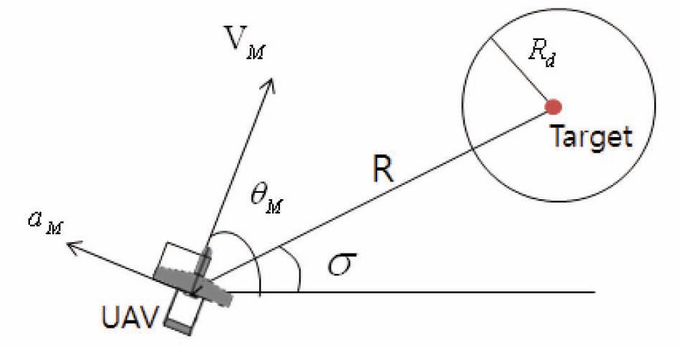
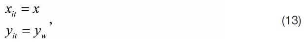
After passing the waypoint, the guidance system will be changed from the pseudo pursuit guidance law, to the distance error dynamics-based guidance law. In this section, the distance error dynamics-based guidance law is briefly summarized [7,8]. Consider a point mass UAV model, as shown in Fig. 7. The following assumptions are required for the distance error dynamics-based guidance law. First, the autopilot and sensor dynamics of the UAV are significantly faster than the UAV dynamics. Second, the velocity of the UAV is constant during loitering. Third, the angle-of- attack (AOA) of the UAV is very small, and may be neglected. Finally, the acceleration vector of the UAV is perpendicular to the velocity vector of the UAV. Then, the equations of motion can be represented as

where,

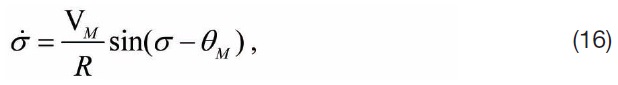
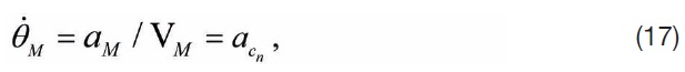
Differentiating eq. (18) with respect to time, once and twice, yields


Using eqs. (15)-(17), the second derivative term of the distance error, eq. (20), can be rewritten as
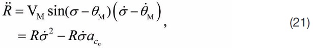
Substituting eq. (20) into eq. (21), we have

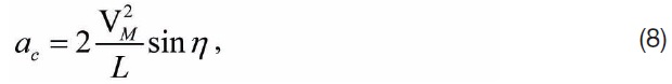
Let us propose a normalized centrifugal acceleration command
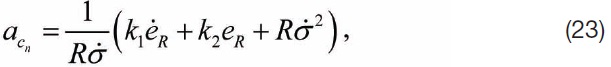
Then, substituting eq. (23) into eq. (22), the distance error dynamics can be represented as

Two guidance gains,
To verify the performance of the proposed guidance law, numerical simulation is performed. The considered mission is the coordinated stationary target observation of multiple UAVs, with the waypoint constraint. The waypoints of the follower UAVs move on the desired observation circle, after the leader UAV passes through its waypoint.
In the numerical simulation, the nominal velocity of each UAV is 14 m/s, and the desired observation radius is chosen as 300m. The initial position of the leader UAV is (0, 0), and the positions of the follower UAVs are (1800, 0) and (-100, 1600), respectively. The target position is (800, 600). The limit of guidance command is chosen as 2
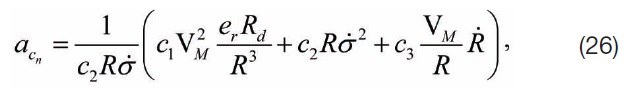
Then, the normalized centrifugal acceleration command of eq. (23) can be rewritten as
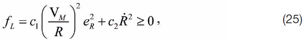
Finally, the first derivative of the Lyapunov candidate function is negative semi-definite.
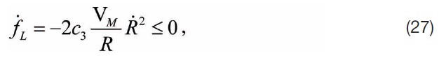
The proposed Lyapunov candidate function is a continuously differentiable function, such that for some
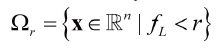
is bounded, and its first derivative is negative semi-definite, where x={
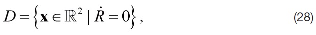
and
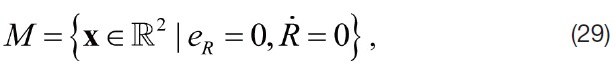
If M contains a point with
Remember that
Figure 8 shows the 2-dimensional flight trajectories of three UAVs, turning around the target counter clockwise. In the CCW turn case, the considered phase angle 1 between the leader UAV (UAV1) and the first follower UAV (UAV 2) is set as 90 degrees, and the phase angle 2 between the leader UAV and the second follower UAV (UAV 3) is chosen as -120 degrees. The initial waypoints (IW) of the three UAVs are represented as square dots in Fig. 8. Once the leader UAV (UAV 1) has passed through its waypoint, the follower UAVs’ waypoints move along the desired observation circle, as shown in Fig. 8. The final waypoints (FW) of the follower
UAVs are described as circular dots. Triangular dots are the positions of three UAVs loitering around the given target at 130 seconds. As shown in Fig. 8, the phase angle differences are maintained.
Figure 9 shows the time history of the phase angle differences and the velocity commands, in the CCW turn case. After all UAVs have passed their waypoints, the phase angles among UAVs maintain the desired values, as shown in Fig. 9. Also, the velocity commands are generated to pass the corresponding waypoint, for maintaining the desired phase angle differences, as shown in Fig. 9.
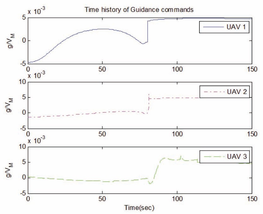
Figure 10 shows the time history of normalized guidance commands in the CCW turn case. In the simulation, the limit of the normalized centrifugal acceleration guidance command is chosen as about 1.4
In the CW turn case, the initial conditions, guidance gains, the nominal velocity of each UAV, and the limit of
the guidance command and the velocity command are the same as in the CCW turn case. And, the considered phase angle 1 between the leader UAV (UAV1) and the first follower UAV (UAV 2) is set as 120 degrees, and the phase angle 2 between the leader UAV and the second follower UAV (UAV 3) is chosen as -90 degrees. Figure 11 shows the 2-dimensional flight trajectories of three UAVs turning around the target clockwise. The triangular dots are the positions of three UAVs loitering around the given target at 200 seconds.
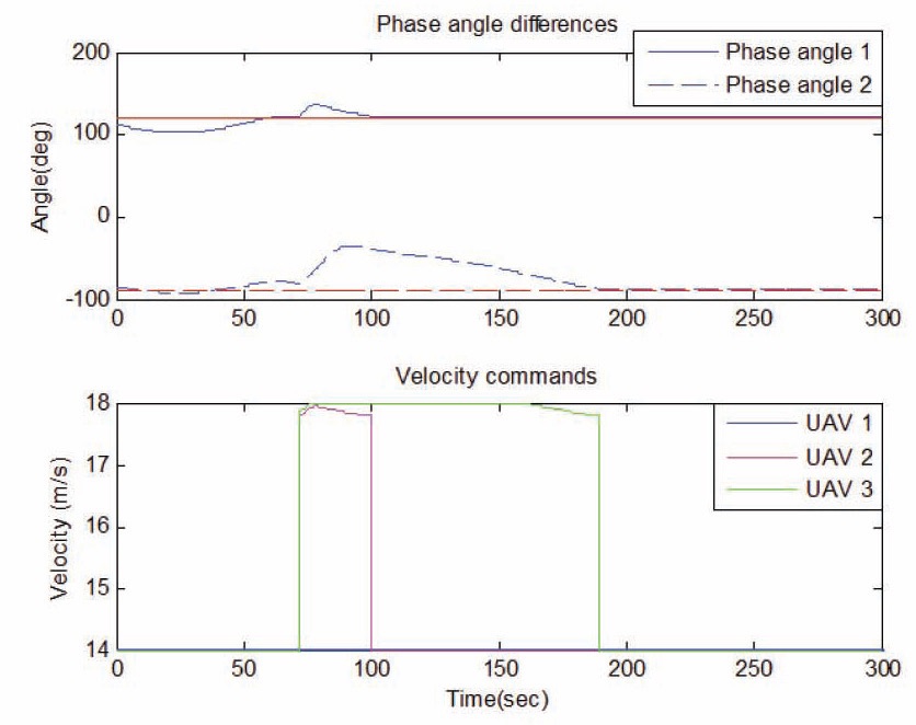
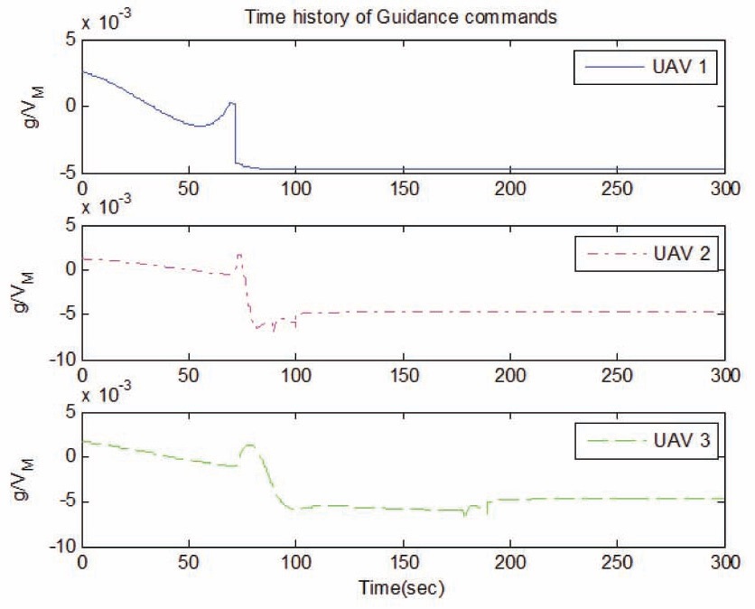
Figure 12 shows the time history of the phase angle differences and the velocity commands, in the CW turn case. Again, the phase angle difference is maintained, as shown in Figs. 11 and 12. Figure 13 shows the time history of the normalized acceleration guidance commands in the CW turn case. As shown in Fig. 13, each normalized acceleration guidance command is below the limit of the normalized guidance command.
Pseudo pursuit guidance law and distance error dynamicsbased guidance law are combined, to perform stationary target observation, considering the waypoint constraint of multiple UAVs. Pseudo pursuit guidance law is used, to satisfy the waypoint constraint. After a UAV has passed through its waypoint on the observation circle, distance error dynamics-based guidance law is used, to loiter around the stationary target. To avoid colliding with the leader UAV, and improve the mission capability, the phase angle difference is considered to determine the waypoints of follower UAVs, and pseudo pursuit guidance law is analyzed geometrically, to guide the UAV to the waypoint. Numerical simulation is performed, to verify the performance of the proposed nonlinear guidance scheme, in the clockwise and counter clockwise turn cases. The proposed guidance law can be used to perform surveillance or fire monitoring mission of small multiple UAVs.