At present, the smart phone camera industry requires a highly precise optical module which consists of a high resolution image sensor and lenses with small F-number. In addition, the depth of focus of the optical module is very short because it is proportional to the focal length of the phone camera lens set and the pixel size of the image sensor, as described in Eq. (1).

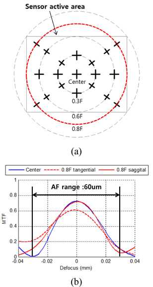
For example, a phone camera consisting of a 1/3” size image sensor with 12 mega pixel and an F/1.8 lens has a depth of focus of only 3.6 μm. Given that the smart phone camera market demands higher resolutions (smaller pixel sizes) and brighter lenses (a short focal length), the depth of focus is becoming shorter with the development of technology. The depth of focus is the amount of the distance between the nearest and farthest objects that appear at an acceptable sharpness, meaning that the image sensor cannot distinguish the resolution performance within the depth of focus [1]. Therefore, the scanning resolution of an actuator to find the focal point should be less than the depth of focus. It is also necessary to establish a proper focusing scan range. Figure 1 depicts the through focus MTF data of an F/1.8 lens at the Nyquist/4 frequency. In order to ensure that the MTF peak is located within a scanning range, the defocus range should be at least ± 30 μm, but a longer range than the simulation data is required (generally twice as long in industry) due to the level of manufacturing tolerance to cover the initial focus position error. The number of focus scanning steps without any optimization will exceed 30, necessitating a long time to evaluate the MTF for each phone camera module. Some customers want to evaluate the MTF of the phone camera module in the low frequency area; in such a case, it will take more time to find the focal point with a longer focus scanning range.
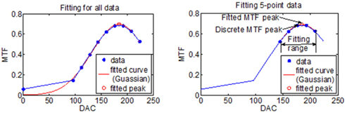
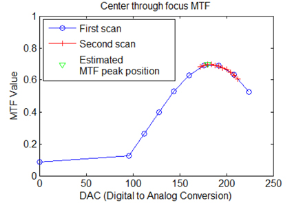
To reduce the number of focus scanning steps, the double-scan method was introduced. In this method, the initial coarse scan roughly finds the approximate MTF peak position and the second fine scan is repeated around the approximately estimated peak position. This previous MTF peak search method is depicted in Fig. 2. In general, the resolution of the first coarse scan is 16 DAC (Digital to Analog Conversion) while the resolution of the second fine scan is 4 DAC, meaning that the resolution of the fine scan is four times better than that of the coarse scan. Given that the sensitivity of the actuator used in this study was 0.5 μm/DAC, the resolutions of the coarse and fine scans were 8 μm and 2 μm respectively, which is less than the depth of focus.
The number of scanning steps of the previous double-scan method is approximately 20 on average, representing a severe limitation of the manufacturing UPH (Unit per Hour). Moreover, the accuracy of the previous method is still not ideal despite the fact that the resolution of the fine scan is within the depth of focus.
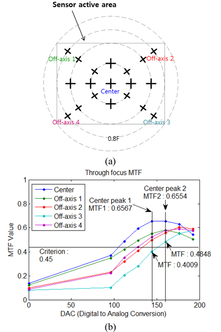
Figure 3 illustrates an inaccurate center MTF peak position as detected by the previous method. The discrete through focus MTF data causes a false MTF evaluation. The amount of the difference between center field MTFs 1 and 2 is negligible; however, the difference in the off-axis MTF between positions 1 and 2 is significant enough to affect the judgement. For example, the off-axis MTF at field position 3 satisfies a criterion associated with the center peak 2 case, whereas it is not in the criterion associated with the center peak 1 case. In order to avoid this mismatched situation, the number of focus scanning steps should increase, but the manufacturing UPH will increase as well. On the other hand, if we reduce the autofocusing resolution to increase the UPH, it will be difficult to find an ideal MTF peak position, leading to false judgements. The goal of this paper is to suggest a reliable means of finding within a short period of time an accurate MTF peak position by a method which can be applied in industrial fields through discrete data fittings. A large amount of manufacturing data was analyzed to demonstrate that the suggested method was safe enough to be implemented in the production processes.
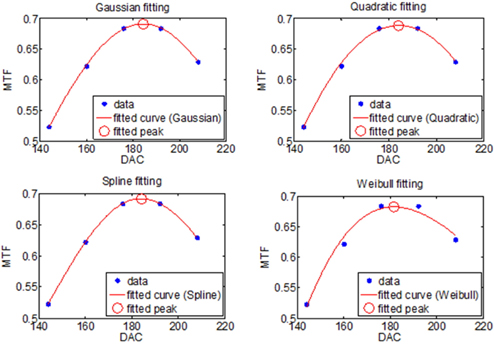
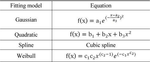
In this paper, four types of fitting models were considered and applied to through focus MTF data, as shown in Table 1 and Fig. 4.
Fitting models
The Gaussian model has three parameters: the amplitude ‘a1’, peak position ‘a2’, and full width at half maximum of the Gaussian function ‘a3’. With this function, it is convenient to find the MTF peak position and value because the parameter ‘a2’ represents the MTF peak position itself and the amplitude ‘a1’ is the MTF value at the peak positon. The polynomial interpolation method was tested with the second degree because high order polynomials yield results similar to those of the spline method as long as instability due to Runge’s phenomenon is eliminated [2]. Commercial optical design software, Code-V and Zemax, were used for the spline fitting. The Weibull model was also tested to verify the asymmetric condition of the through focus MTF curve, as shown in Fig. 4 (d) [3, 4]. Only five data points from the coarse scan were used around the MTF peak position to compare the performances of these four fitting methods, as described in Fig. 5.
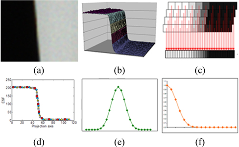
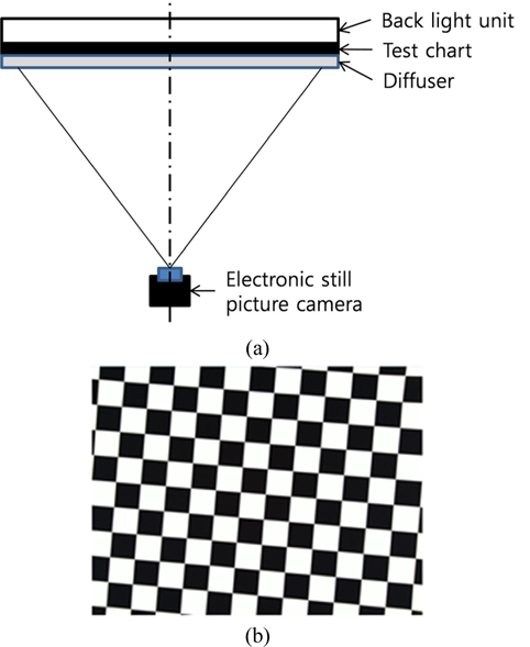
The MTF test environment followed ISO-12233, except for the replacement of a reflection chart with a transmittance chart [5]. The back light level was controlled such that it exceeded 200 cd/m2, with 10% uniformity across the entire chart. The test chart was designed as a seven degree slanted edge checker box, as shown in Fig. 6.
MTF calculation also referred to ISO-12233. The calculation sequence and algorithm are described in Fig. 7.
The SFR (Spatial Frequency Response) was obtained from the normalized DFT (Discrete Fourier Transform) of the LSF (Line Spread Function), as expressed by Eq. (2) [6, 7].
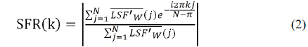
In Eq. (2), k represents the normalized spatial frequency. Before the DFT, the hamming window W was multiplied by the LSF to reduce the effects of noise by reducing the influence of pixels at the extremes of the window, which had some response due to noise but little response due to the image edge located at the center for the window [5]. The LSF was calculated from the derivative of the ESF (Edge Spread Function), as shown below
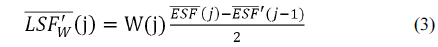

In Eq. (4), a four-fold super-sampling scheme with binning was adopted to estimate the ESF to increase its accuracy [8].
III. EXPERIMENTAL RESULTS AND STATISTICAL ANALYSIS
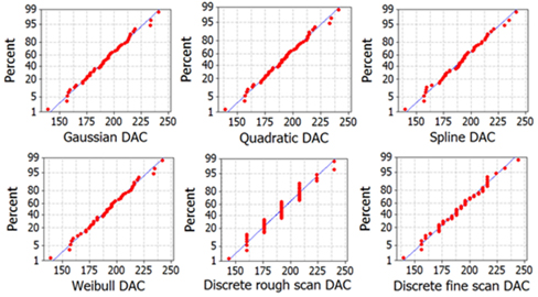
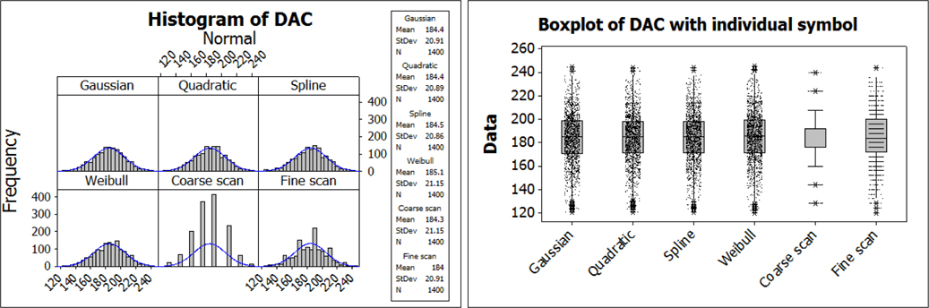
A statistical analysis was conducted to demonstrate the feasibility of our study with a sampling number of 1,400 modules. The experimentally obtained MTF peak position was expressed with the DAC (Digital to Analog Conversion) value, as shown in Fig. 8, because the DAC was directly determined from the driver IC (Integrated Circuit) signal for the autofocusing actuator of the phone camera module [9, 10]. Normality tests of the peak position were performed for all six methods: the four fitting methods, the coarse scan only, and the previous double-scan (coarse + fine) case. At this time, based on the central limit theory, there was no reason to check the degree of normality because the sample size was large enough. Therefore, 50 random samples were selected to perform the Anderson-Darling normality test [3, 4].
According to Table 2, especially considering the Anderson-Darling result and p-value, the MTF peak position found by the coarse scan was not normal because the p-value was less than 0.05, establishing the validity of the alternative hypothesis, whereas the remaining five methods satisfied the normality test. It should be note that the Anderson-Darling results and the p-value of the previous double-scan method were acceptable but relatively worse than those of the fitting methods, meaning that the result of this study suggests the possibility of the elimination of the second fine scan through the use of the fitting models on the first coarse scan data in order to find the MTF peak position. Normally, it took an average of 526 ms for each focusing step. Calculating 1,400 instances of log data of the samples (phone camera modules), the number of steps in the coarse scan was 10 in average value, while for the fine scan the average was 11. As a result, 21 in total autofocusing steps were required for the previous double-scan method, indicating that it took 11.05 s per phone camera module. With the fitting models, however, the fine scan time could be reduced. The calculation time for data fitting was negligible compared to the fine scan time. Of course, the off-axis MTF at the new focusing position should be considered. In actual experiments, the fitting methods could reduce 2.7 s per phone camera module, while the manufacturing UPH value was improved from 310 to 404. Moreover, the individual plot and histogram shows that the peak position determined by the previous double-scan method remains discontinuous, whereas the fitting methods can find a more accurate MTF peak position between discrete data instances, as shown in Fig. 9.
[TABLE 2.] Normality result and basic statistics
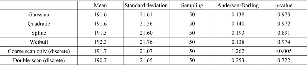
Normality result and basic statistics
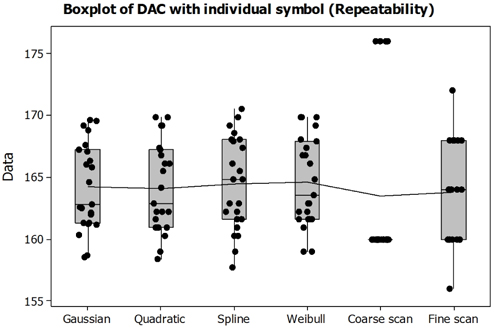
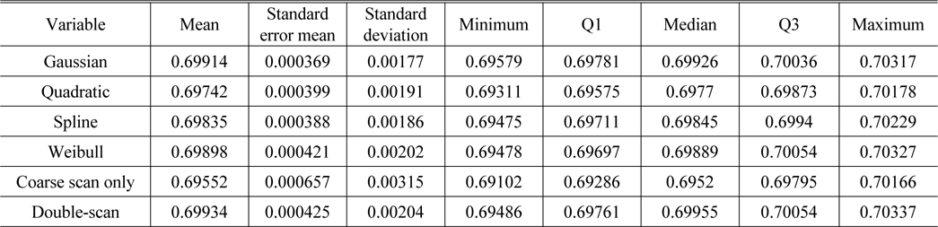
One sample was selected and tested 23 times repeatedly. The results shown in the descriptive statistics reach similar conclusion. The standard error of the mean and the standard deviation of each method are displayed in Table 3. All four fitting methods showed no significant differences between them, also showing a slightly better score than the previous double-scan method. The coarse scan only case showed relatively poor score in our study, as shown in Fig. 10. By comparing the MTF value (not the MTF peak position) for each approach, differences between 6 methods did not appear, as described in Table 4.
[TABLE. 3] Descriptive statistics for repeatability of the MTF peak position
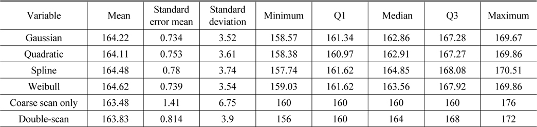
Descriptive statistics for repeatability of the MTF peak position
[TABLE 4.] Descriptive statistics for repeatability of the MTF value at the peak position

Descriptive statistics for repeatability of the MTF value at the peak position
In a manufacturing system, it is hard to satisfy both performance and capability at the same time. To overcome this limitation, four fitting methods were tested with 1,400 phone camera modules, and we suggest a way of increasing both capability and performance (more accurate MTF peak position than the previous double-scan method). By analyzing numerous instances of mass production log data, we verified that all four fitting models were reliable enough to be applied to mass production processes.


![(a) Field information [10], (b) Through focus MTF data. An F/1.8 lens at the Nyquist/4 frequency requires a scanning range of at least 60 μm.](http://oak.go.kr/repository/journal/20781/E1OSAB_2016_v20n1_150_f001.jpg)
![(a) Field information [10], (b) MTF variation with an inaccurate center peak detection.](http://oak.go.kr/repository/journal/20781/E1OSAB_2016_v20n1_150_f003.jpg)