Free-space optical (FSO) communication is an advanced technology to implement line-of-sight transmission of light signals. It transmits laser carrying signals through a free-space channel with high capacity, high bandwidth, and a flexible network [1]. FSO is one of the most promising alternative schemes for addressing the ‘last mile’ communication bottleneck in emerging broadband-access markets [2]. However, atmospheric disturbance can easily affect the laser beam. The refractive index of the atmosphere changes randomly because of variations in temperature, humidity, and wind speed in the atmosphere. This will lead to beam wandering, scattering, scintillation, and power fluctuations [3]. The phase and intensity of the laser are distorted, and the coupling efficiency decreases [4, 5]. Consequently the bit error rate (BER) of the communication system is degraded. This arouses the interest of researchers worldwide in studying phase correction, and effective methods are in high demand for FSO communication systems.

Adaptive optical (AO) systems have been successfully applied to FSO to compensate the distorted wave front [3-9]. Based on the phase-conjugation principle, traditionally there are two main branches. One in [6] is based on a wave-front sensor, such as the SH-WFS, to detect the local slope of the wave front and reconstruct the wave front in the Zernike or some other model. With a model, a deformable mirror (DM) can be controlled to construct a conjugated wave front, to offset the aberrations and obtain an approximately planar wave. In this method, the computational cost is very high for large numbers of subapertures in the sensor. Therefore the typically used sensors will fall short when high speed of detection and correction are needed, to implement fast adaptive optics in the FSO system. The other branch is the wave-front sensorless optimization method [3, 9], which aims to optimize the performance metrics of the received laser, such as Strehl ratio (SR), root mean square (RMS) and image sharpness functions, etc. The AO system searches for the suitable voltage to control the DM to optimize the performance metric. Many algorithms, such as simulated annealing (SA), hill climbing, and stochastic parallel gradient descent (SPGD) have been developed [5]. Among them, the SPGD algorithm is widely considered for its simple mechanism and rapid convergence, although hundreds of iterations are needed.

Recently, some new methods have been proposed. Reference [7] proposes a method to process Shack-Hartmann data by a focal-plane approach. This method is more favorable in noise propagation, compared to classical Shack-Hartmann, and senses more phase modes with fewer subapertures under a comparable computation burden. A phase-retrieval method is used instead of the wave-front-slope method to reconstruct the wave front in reference [8]. The method provides more accurate estimation of aberrations in nearly flat wave fronts. Interestingly, reference [10] proposes a combined approach involving SPGD and DM-model-based algorithms, to achieve similar correction results to those of SPGD with many fewer iterations. But in this method a SH-WFS is not effective, and both SPGD and DM-model-based algorithms need parameter settings that will increase the complexity of the method. In addition, a trust-region method has been proposed that is superior to both SA and SPGD algorithms, with respect to convergence rate for slowly changing wave-front aberrations, in reference [11].

Considering the rapidly changing atmospheric environment in an FSO system, we propose an HC scheme for wave-front corrections. This method combines the DG method [12] and SPGD algorithm to improve both the results of wave-front compensation and convergence rate.

This paper is organized as follows: In section II, the principles of the DG method and SPGD algorithm are briefly introduced and their deficiencies discussed, then we propose an HC scheme based on a suitable combination of the methods discussed above. In section III, computer simulations using MATLAB are carried out and the results are analyzed, to investigate the compensation capability of the HC scheme. Finally, we give our conclusion in section IV.

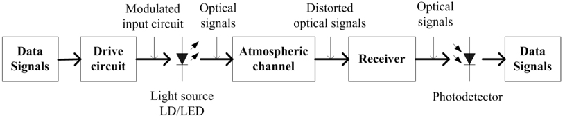
The fundamental scheme of FSO communication is shown in Fig. 1. We adapt optical intensity modulation, and the data signals directly modulate the light source to generate optical signals. When the optical signals are transmitted to an atmospheric channel, they may suffer from atmospheric turbulence, and the receiver may receive optical signals with distorted wave fronts. Therefore, at the receiver we use an AO system to compensate for the aberrations of the distorted wave front. Then the optical signals with corrected wave fronts are coupled into the fiber and detected by the photodetector, to recover the original data signals.

As we know, a wave front distorted by atmospheric turbulence is commonly described by the Zernike polynomials [13], which are a set of polynomials defined on a unit circle. It is convenient to use polar coordinates, so that the polynomials are a product of angular functions and radial polynomials. The wave front is described as [14]

where (r, θ) are the polar coordinates of the pupil, Z_i(r, θ) is the ith order Zernike polynomial, ai is the ith coefficient, and q is the highest order Zernike polynomial considered. The expression ϕ(r, θ) can be transformed into rectangular coordinates ϕ(x, y) for calculation.

To compensate a distorted wave front, the DG method is frequently used to detect and calculate a wave-front gradient matrix G using SH-WFS and the optimal control V of DM, which is the least-squares solution of

where G = [G_1x, G_2x, ⋯, G_Mx, G_1y, G_2y, ⋯ G_My,]^T contains the local slopes in the horizontal direction x and vertical direction y, detected in every subaperture, and the subscript M is the number of subapertures of the SH-WFS. The matrix K = (G₁, G₂, ⋯, G_N) is defined as the gradient response matrix of the DM, and N is the number of control elements of the DM.

For later use, we give a brief interpretation of Eq. (2). We suppose that the voltages applied to the actuators of the DM are linear, and let Ψ(x, y) be the wave front generated by the N actuators, i.e.

where (x, y) are the coordinates of the wave front generated by the DM and I_n(x, y), n = 1, 2, ⋯, N is the influence function [5] of the n th actuator, and

where (x_n, y_n) are the central coordinates of the nth actuator, ω is the coupling coefficient, b is the normalized interval between the adjacent actuators, and α is the Gaussian index.

On the other hand, the mean local gradient of the distorted wave front in the mth (m=1, 2,⋯, M) subaperture is regarded as the mean of the partial derivative of the wave front ϕ(x, y) in the area S_m, which is the local area of the m th subaperture [6]. Based on Eq. (3) and (4), we obtain

where

Since this method directly calculates the optimal control voltage by the gradient of the wave front, without wave-front reconstruction, it can reduce the computational cost of the AO system. From Eq. (2) we can see that the influence function of DM is a key factor in compensation. To investigate the compensation capacity of the DM, we introduce the definition of compensation error as

where RMS_o is the RMS value of the original distorted wave front, and RMS_c is the RMS value of the corrected wave front. To test the general correction ability of the DM, the first 35 Zernike polynomials are taken as the targets for the correction, and all of their amplitudes are normalized. Here we consider a DM with 61 elements for the analysis. The compensation error of the 61-element DM for each Zernike order from 3 to 35 is shown in Fig. 2. From this figure, we can see that the compensation error increases with increasing Zernike order, which means the DG method is relatively incapable of correcting high-order aberrations.

For this reason, we introduce the SPGD algorithm for the sensorless wave-front compensation given in [3] to correct high-order aberrations. In this algorithm the object of optimization is a performance metric J for the received laser. This algorithm searches for optimal control u = (u₁, u₂, ⋯, u_N) and obtains the optimal J iteratively. In addition, the SPGD controller generates a set of statistically independent control perturbations {δu_j^(k)}, j = 1, 2, ⋯, N for each iteration k to update the control u. The search procedure is carried out as follows:

where

and γ is the gain coefficient. If the objective of optimization is to achieve the maximum value of J, then γ is positive, else γ is negative.

For SPGD, given γ and J, the gradients of the wave front follow the direction of descent with iterations. When the atmospheric disturbance increases, leading to a more distorted wave front, the correction by the SPGD algorithm will act to reduce this distortion.

Considering the effect of increasing convergence rate on the correction and the performance metric, we make use of the mature technologies of the DG and SPGD algorithms to propose an HC scheme based on a combination of the properties of these methods. For a distorted wave front, the DG method can compensate low-order aberrations without iteration, while the residual wave front consisting of a large proportion of high-order aberrations will be compensated by SPGD. In this way, the initial wave front corrected by SPGD is a less distorted wave front, with a smoother phase plane than the wave front of the inserted laser, which means much fewer iterations are needed to reach convergence. Moreover, our proposed HC scheme uses the SH-WFS to compensate the low-order aberrations, so that the accuracy requirement for the sensor is reduced, and we do not have to choose a SH-WFS with many subapertures. Large number of subapertures will divide the inserted laser power into many small parts, which causes difficulties in CCD detection. Furthermore, the computation pressure is relieved, since the size of G is 2M×1, which is proportional to the number of subapertures.

In this paper, we adapt a hybrid scheme by combining the mature schemes of the DG method and SPGD algorithm. The functional blocks are diagrammed in Fig. 3, in which the wave-front corrector is the DM shared by the Direct-Gradient Block and SPGD Block. The main process of this scheme is given as follows.

(1) When the light arrives, the Algorithm Selection Block identifies whether the inserted wave is the original, distorted wave or the residual wave, then selects the corresponding correction block. (2) If it is the original, distorted wave, the Direct-Gradient Block begins to detect the wave-front-gradient matrix G and calculates V of DM using Eq. (2). (3) The wave-front corrector generates a conjugated wave front to compensate the original wave front, and a residual wave is output. (4) The residual wave propagating back to the Algorithm Selection Block, is switched to the SPGD Block, and then iteratively corrected based on Eq. (8). With the SPGD algorithm, the wave front is iteratively corrected until the value of the performance metric J converges. (5) After correction, the optimized wave is coupled into the single-mode fiber and processed by the receiver. A diagram of this entire process is presented in Fig. 4.

For FSO, the coupling efficiency of the signals inserted into the fiber in the receiver has significant influence on system performance [15]. Thus in the SPGD block the performance metric J is set equal to the SR, which is the ratio of the distorted laser’s peak intensity to that of the ideal laser. As shown in Eq. (11) [16], SR is an estimation of the coupling efficiency and can directly reflect the aberration effect

where A_r(f) is the Fourier transform of the single-mode fiber's optical field and f is the frequency of the optical wave. The coupling efficiency increases as SR improves.

On the other hand, the BER of FSO communication links with on-off keying systems increases as RMS rises [17]. The relationship between RMS and SR is expressed as [16]

This means that the BER decreases with increasing SR. In other words, improvement of SR both increases coupling efficiency and reduces BER.

In the following section, by observing the SR of the system with our proposed compensation scheme, we present simulation results and analysis of wave-front compensation, to investigate the performance of our HC algorithm.

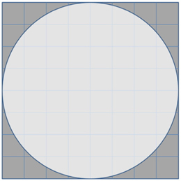
In our simulations, for the Direct-Gradient Block we use the SH-WFS with an 8×8 subaperture array, in which the subapertures are not considered in every corner of the array shown in Fig. 5, to avoid detection difficulties in low light [6]. For the SPGD Block, the perturbations {δu_j} obey a Bernoulli distribution with probability 0.5 each for δu = +σ and δu = -σ. We define γ = γ₀ /(J + C), where C is a constant to avoid too large γ when J is sufficiently small. Parameter settings for the SPGD algorithm and HC method are the same in our simulations. The wave-front corrector is a DM containing 61 control elements, to realize a trade-off between an accurate influence function and a suitable aperture size in the FSO system. The arrangement of the 61 actuators is shown in Fig. 6.

The distorted wave front that we introduce is the superposition of Zernike polynomials with coefficients a_i listed in Table 1, where a_i is set by the covariance matrix of Zernike terms [14]. We define the coefficient vector A = [a₁, a₂, ⋯, a₂₀]^T and use the covariance matrix (Eq. (4) in [14]) to evaluate A according to Eqs. (8), (12), and (13) presented in [14]. The SR of the distorted wave-front is 0.1668.

Using this distorted-wave-front sample, we first simulate the DG method; after correction, the corresponding SR increases to 0.6958. The SRs of the iteratively corrected residual wave fronts are given in Fig. 7. From this figure, we can see that this method cannot further improve SR with increasing iterations, for high-order aberrations. Thus in our HC scheme the correction is carried out only once, to compensate the low-order aberrations with the DG algorithm and the high-order aberrations with the SPGD method.

Next we conduct the simulation of our HC scheme and compare its performance to that of the SPGD algorithm in correcting the original, distorted wave front. The improvements in SR for the HC and SPGD algorithms are presented in Fig. 8. We find that the HC scheme can converge much faster than the SPGD algorithm. In Fig. 8, when the SR is 0.8 the SPGD algorithm requires 144 iterations, but the HC scheme only needs 21. When the SR becomes 0.9, the number of iterations is about 370 by SPGD, while 110 by the HC scheme. Since the low-order aberrations have been corrected, the SR increases to 0.6958, so that further corrections implemented by the SPGD method need much fewer iterations.

Figure 9 shows the differences of the phase plane before and after correction. Figure 9(a) is the original, distorted wave front (SR=0.1668). It is obvious that it becomes flatter after correction by DG (SR=0.6958), as shown in Fig. 9(b), and it gets smooth after correction by the HC scheme (SR=0.9), as shown in Fig. 9(c). The range of the wave front narrows correspondingly.

Furthermore, we discuss the intensity characteristics of the laser beam to investigate the improvement of the coupling efficiency. The intensity I(x, y) is normalized to the peak intensity of the ideal plane wave, where the coordinates (x, y) identify a pixel in the focus plane of the detector. Figure 10 shows the normalized intensity of the original, distorted light, the DG-corrected light, and the HC-corrected light. The peak intensity rises from 0.1098 to 0.4319 after correction by the DG method. With correction by the HC scheme, when SR is 0.9 in Fig. 9(c) the peak intensity is 0.5549, as shown in Fig. 10(c). This illustrates that the HC scheme can enhance the light's intensity by almost a factor of 5. With the increase in SR, more signal power will be coupled into the single-mode fiber so that the coupling efficiency increases, which helps the FSO system to correctly detect the signals.

To verify the compensation effect of the HC scheme, besides the wave front discussed above, we introduce another seven wave fronts, simulated by Zernike polynomials with different maximum Zernike orders q(q = 20, 25, 30 and 35) and defined as ϕ₁, ϕ₃-ϕ₈ respectively. The wave front already discussed is ϕ₂. The initial SRs of the eight distorted-wave-front samples ϕ₁~ϕ₈ are 0.1604, 0.1668, 0.0493, 0.3072, 0.1064, 0.1667, 0.0120, and 0.3760 respectively. We compare the compensation effect of the DG method, SPGD algorithm, and HC scheme for every sample, to get a clear picture of the HC scheme. The improvements in SR with the SPGD and HC schemes of the eight samples ϕ₁-ϕ₈ are shown in Fig. 11.

From Fig. 11 we can see that the HC scheme is obviously superior to the SPGD algorithm, because it converges more rapidly than SPGD for every sample, especially for samples ϕ₃ and ϕ₇ with quite low initial SR. As shown in Figs. 11(c) and (g), by correction with SPDG, when SR is lower than 0.1 the rate of SR improvement with iterations is quite low, but the curve becomes much steeper beyond SR=0.1. This means that the correction speed of SPGD is relative to the value of SR. Since low-order aberrations make up a large fraction of the wave-front aberrations, it is difficult for SPGD to correct the low-order aberrations. The HC scheme can compensate the low-order aberrations by the DG-Block; thus it increases the correction speed of SPGD. Additionally, our HC scheme provides higher SR than the SPGD algorithm within 1000 iterations.

Next we will perform a numerical analysis of the results. We define J_O as the SR of the original, atmospheric distorted wave front, and J_DG as the SR of the residual wave front after correction by the DG method. J_H and J_S are respectively the correction results of the HC and SPGD algorithms after 1000 iterations, as shown in Fig. 10. Furthermore, k_H^0.8 and k_S^0.8 are the minimum iteration numbers that the HC scheme and SPGD algorithm need respectively for SR to reach 0.8. The simulation results for the eight samples are presented in Table 2, which significantly shows that for every sample the HC scheme can reach much higher SR than the DG method, especially for samples ϕ₅-ϕ₈ with higher Zernike orders. This verifies that the HC scheme can utilize the SPGD algorithm to offset the deficiency of the DG method in high-order aberration correction.

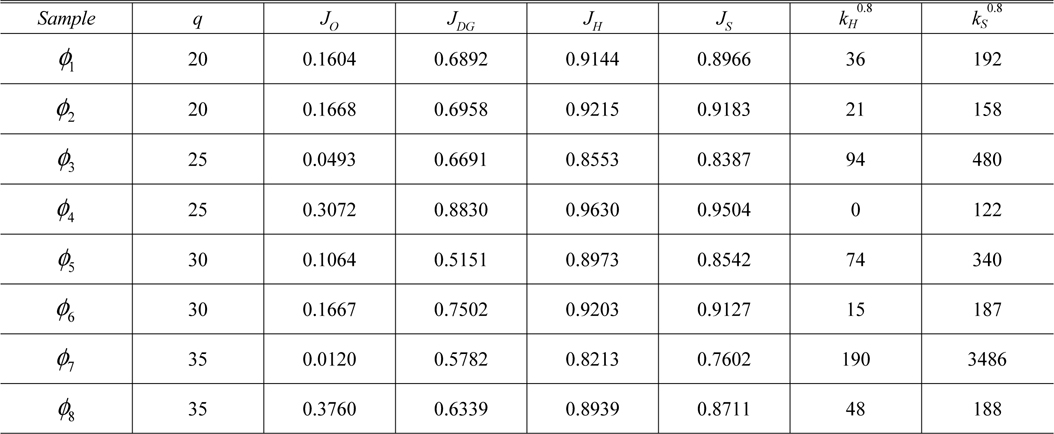
To obtain convenient comparisons of correction results for different samples, we define the indice of the correction effect of the HC scheme as η and the indice of its correction speed Δk^0.8, precisely

For the samples enjoying better corrections by our HC scheme, η is larger, and for the samples with faster correction by the HC scheme than by SPGD, Δk^0.8 is larger. The indice values for the eight samples are shown in Table 3.

As shown in Table 3, for samples of the same Zernike order, those with lower initial SR can realize higher η and Δk^0.8. For example, for samples ϕ₅ and ϕ₆ simulated by 30 Zernike polynomials, the initial SRs are 0.1064 and 0.1667 respectively, η are 7.43 and 4.52, and Δk^0.8 are 266 and 172. The results keep consistent for other samples. This means that under the same wave-front simulation conditions, the HC scheme can perform better at compensation of wave fronts with more severe aberrations. This benefits from the DG-Block’s compensation, because the DG method plays an important role in compensating the low-order aberrations. By DG-Block correction, the initial wave front for the SPGD algorithm to correct is smoother and the SR increases, since the correction speed of SPGD depends on the value of the SR.

In summary, from simulations of different distorted wave fronts and the analysis of the results, we know that through a suitable combination of the DG method and the SPGD algorithm our HC scheme can achieve higher performance metrics than that of the DG method and convergent faster than the SPGD algorithm when low-order aberrations are compensated in advance by the DG method. After correction by the HC scheme, SR increases, so that the light intensity increases and more power is transmitted to the receiver, for higher coupling efficiency and improved communication quality.

In this paper we have proposed a hybrid-method HC scheme to compensate wave-front distortions resulting from the turbulent atmosphere in FSO communication. This scheme reduces the computational complexity of the compensation process and accelerates the convergence of the performance metric, to adapt to the real-time requirements of FSO communication. Based on the distorted wave fronts generated by Zernike polynomials, we compare the compensation performance of the SPGD algorithm, DG method, and our HC scheme by computer simulations. We find that with the SPGD-Block’s correction our HC scheme can achieve higher SR than the DG method, especially for wave fronts with higher Zernike orders. And the HC scheme can increase the correction speed of SPGD by increasing SR in the DG-Block, especially for severely distorted wave fronts, because high SR requires fewer iterations than low SR does. Our method can help an FSO system to improve coupling efficiency of the laser to the receiver and decrease BER.