Identification and Determination of Oil Pollutants Based on 3-D Fluorescence Spectrum Combined with Self-weighted Alternating Trilinear Decomposition Algorithm

Cheng
Pengfei; Wang
Yutian; Chen
Zhikun; Yang
Zhe

doi:10.3807/JOSK.2016.20.1.204

OA학술지
Journal of the optical society of Korea

Identification and Determination of Oil Pollutants Based on 3-D Fluorescence Spectrum Combined with Self-weighted Alternating Trilinear Decomposition Algorithm

DOI : 10.3807/JOSK.2016.20.1.204
Author: Cheng Pengfei, Wang Yutian, Chen Zhikun, Yang Zhe
Publish: Journal of the optical society of Korea Volume 20, Issue1, p204~211, 25 Feb 2016

ABSTRACT

Identification and Determination of Oil Pollutants Based on 3-D Fluorescence Spectrum Combined with Self-weighted Alternating Trilinear Decomposition Algorithm

KEYWORD

SWATLD , 3-D fluorescence spectrum , Oil mixture , Component number

본문

Collapse all

I. INTRODUCTION

Oil pollution seriously threatens the safety of human and ecological environment. Measuring oil pollutants has become an urgent problem [1]. Fluorescence detection has the advantages of good selectivity and high precision [2-5]. D. Patra applied three-dimensional fluorescence spectrometry to identify diesel with trace amounts of kerosene and gasoline, obtaining good result [6]. R. J. Kavanagh used synchronous fluorescence spectra to measure a variety of polycyclic aromatic hydrocarbons in water, and to successfully distinguish the type of polycyclic aromatic hydrocarbons [7]. Polycyclic aromatic hydrocarbons usually have stronger fluorescence properties [8-13], and the fluorescence spectra of oil pollutants are formed by the superposition of various aromatic hydrocarbon fluorescence spectra. It is relatively difficult to identify the type and determine the content of each component of oil mixture using chemical methods [14, 15]. The parallel factor (PARAFAC) analysis method is a kind of iterative three-dimensional matrix decomposition algorithm, which adopts the alternating least squares principle. It can quantitatively measure the specific components in the existence of interferents [16-18]. But only estimating the component number correctly can we get the accurate result [19, 20]. The self-weighted alternating trilinear decomposition (SWATLD) algorithm, which has been developed in recent years, is insensitive to component numbers, requires fewer iterations and has high stability [20-22]. Hu and Yin applied PARAFAC-alternative least squares (PARAFAC-ALSs) and SWATLD to measure Vancomycin and Cephalexin in human plasma, the experimental result showed that SWATLD algorithm had good effect on the determination of complex analysis of drugs in plasma [23]. Zhang and Wang determined Sulfonamides in synthetic samples and pharmaceutical tablets using SWATLD, showing that SWATLD algorithm can be easily performed and applied to solve second-order calibration problems quickly and accurately [24].

II. THEORIES

   2.1. PARAFAC Model

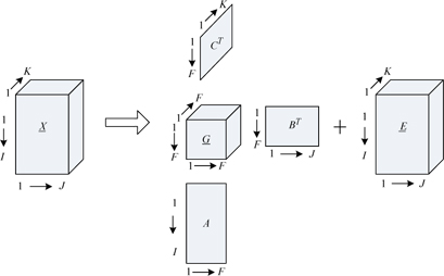
The PARAFAC model means a three-dimensional data matrix can be decomposed into three two-dimensional loading matrices A, B and C. The decomposition algorithm is shown in Fig. 1.

[FIG. 1.] The decomposition diagram of PARAFAC model.

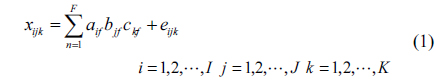
In Fig. 1, is a three-dimensional data matrix, with the sizes of I×J×K. is a three-dimensional core matrix, with the sizes of F×F×F. In the cubical matrix , the super diagonal elements are 1, other elements are 0.

The PARAFAC model formula is expressed as:

The PARAFAC model has specific and actual chemical significance in three-dimensional fluorescence analysis. Scan the I samples in the range of J emission wavelengths and K excitation wavelengths, the I excitation-emission matrices will be produced. Then the I excitation-emission matrices can constitute a three-dimensional matrix sequentially, which corresponds to the formula (1). Here, x_ijk is the element of , standing for the fluorescence intensity of the ith sample in the jth emission wavelength and the kth excitation wavelength; a_if is the element of A, standing for the concentration of the fth factor in the ith sample; b_jf is the element of B, standing for the fluorescence intensity of the fth factor in the jth emission wavelength, so the matrix B can be used to estimate the emission spectrum; c_kf is the element of C, standing for the fluorescence intensity of the fth factor in the kth excitation wavelength, so the matrix C can be used to estimate the excitation spectrum; F is the column number of the loading matrix, standing for the number of the components, namely, it is the number of principal components in the samples; e_ijk is the element of , standing for the residual value that is caused by noise or other unexplained variations.

The PARAFAC analysis algorithm takes advantage of the Alternating Least Square (ALS) method to decompose the three-dimensional matrix , aiming to minimize the sum of squared residuals [25]:

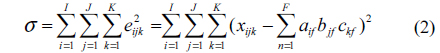
Where, σ is the sum of squared residuals; F is the component number.

   2.2. SWATLD Algorithm

The PARAFAC algorithm has been widely used in the analysis of a three-dimensional fluorescence spectrum, while it is sensitive to component number, and the component number should be estimated accurately. Selecting the correct component number might get the good result. Therefore, a lot of improved PARAFAC algorithms are developed, among which, the SWATLD algorithm has the advantages of insensitivity to component number, fewer iterations, fast operation, good stability, etc.

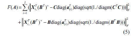
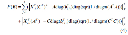
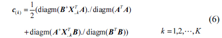
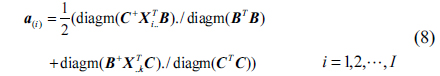
The SWATLD algorithm is the improvement of the PARAFAC algorithm, and it optimizes the three objective functions which are close in internal relation but not completely equivalent. The functions are as follows:

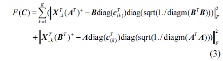
Where, ||.|| represents the Frobenius matrix norm, ./ denotes array division.

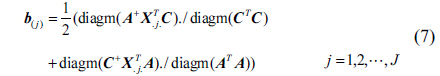
After iterating the formula (3)~(5), we can obtain the following formula:

First, initialize A and B, then calculate C, B and A according to formula (6), (7) and (8), repeat iteration until convergence, the convergence criteria is :

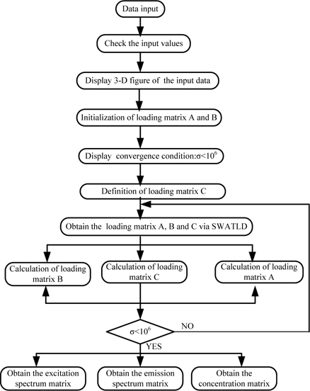
The process of the SWATLD algorithm is shown in Fig. 2.

[FIG. 2.] Process flow chart of SWATLD.

III. EXPERIMENT AND DISCUSSION

   3.1. Experiment Setting and Sample Preparation

The Edinburgh Instruments FLS920 full-function type fluorescence spectrometer is used as the fluorescence detector. The width between excitation and emission slit is 1.11 mm, spectral resolution 2 nm, integration time 0.1s, the excitation wavelength 250~400 nm, fluorescence emission wavelength 270~500 nm, each step length 5 nm. The starting emission wavelength lags the starting excitation wavelength 20 nm to avoid the interference of Rayleigh scattering. Measure the three-dimensional fluorescence spectrum of solutions twice and deduct the background spectrum of solvent to eliminate the effect of Raman scattering.

#97 gasoline and #0 diesel, and ordinary kerosene are the pollutants under test, sodium dodecyl sulfate (SDS) micellar solution is as the analysis of pure sample. The solubility of oil in the water is very low, which reduces the accuracy of the determination. As the solvent of oily substances, the SDS micellar solution can increase the fluorescence intensity of oil in the water, which is widely used in fluorometric analysis [26, 27].

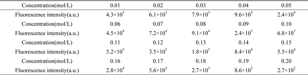
Firstly, prepare the SDS solution. Weigh the different quantities of SDS, and make 20 sets of SDS solution in deionized water, then add 0.05 g kerosene to each. Measure the fluorescence intensity of 20 sets of kerosene SDS solution, which is shown in Table 1. The results show that when the concentration of SDS is 0.1 mol/L, fluorescence intensity of the kerosene SDS solution is the largest, so we choose 0.1mol/L SDS solution as solvent.

[TABLE 1.] The concentration of SDS micellar solution and the fluorescence intensity of kerosene SDS micellar solution

The concentration of SDS micellar solution and the fluorescence intensity of kerosene SDS micellar solution

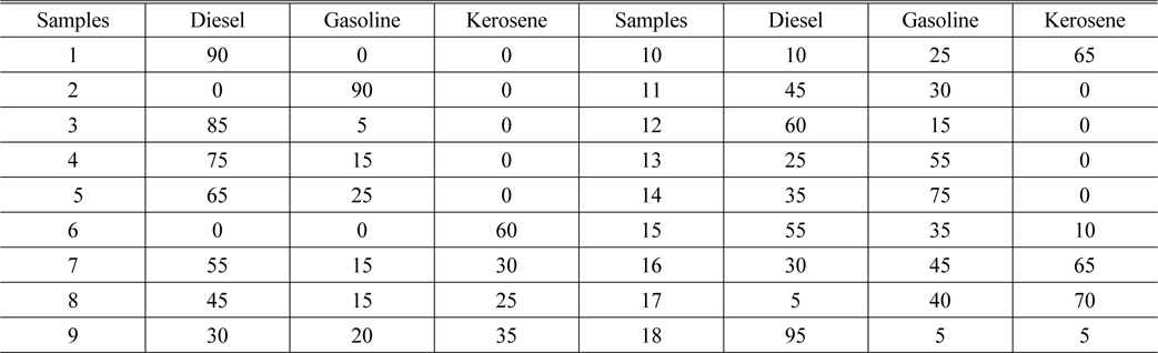
Prepare the 18 samples with different concentrations, and mark them. #1 ~ #10 are the calibration samples, and #11 ~ #18 are the prediction samples. The concentration in each sample is shown in Table 2.

[TABLE 2.] The oil concentration in each sample (mg/L)

The oil concentration in each sample (mg/L)

   3.2. Three-dimensional Fluorescence Spectra

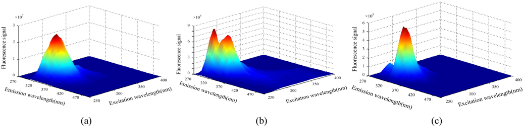
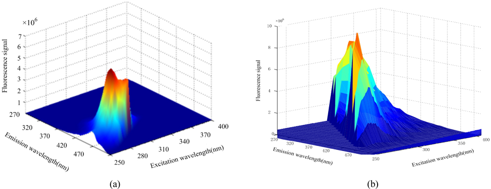
Figures 3(a), (b), (c) show the three-dimensional fluorescence spectra of diesel, gasoline and kerosene solutions respectively. Figure 5 shows the three-dimensional fluorescence spectra of two or three kinds of oil mixture solution. Although the fluorescence intensity of the oils are not identical, two or three kinds of mixed oil seriously overlap spectrally. It is difficult to separate the spectra and predict the concentration.

[FIG. 3.] 3-D fluoresence spectra of three standard samples. (a) 3-D fluoresence spectrum of diesel standard sample. Concentration: 10 mg/L; Width between excitation and emission slit: 1.11 mm; Excitation and emission step length: 5 nm; (b) 3-D fluoresence spectrum of gasoline standard sample. Concentration: 50 mg/L; Width between excitation and emission slit: 1.11 mm; Excitation and emission step length: 5 nm.; (c) 3-D fluoresence spectrum of kerosene standard sample. Concentration: 10 mg/L; Width between excitation and emission slit: 1.11 mm; Excitation and emission step length: 5 nm.

[FIG. 4.] 3-D fluoresence spectra of mixed samples. (a) 3-D fluoresence spectrum of a mixed solution of diesel and gasoline. Concentration of diesel and gasoline is 10 mg/L and 10 mg/L, respectively. Width between excitation and emission slit: 1.11 mm; Excitation and emission step length: 5 nm.; (b) 3-D fluoresence spectrum of a mixed solution of diesel, gasoline. and kerosene. Concentration of diesel, gasoline and kerosene is 10 mg/L, 10 mg/L and 10 mg/L respectively. Width between excitation and emission slit: 1.11 mm; Excitation and emission step length: 5 nm.

[FIG. 5.] Core consistency value of .

   3.3. SWATLD to Mixed Solution of Diesel and Gasoline

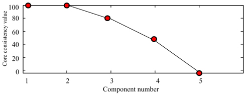
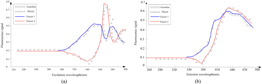
Scan the calibration samples #1 ~ #5 and prediction samples #11 ~ #14 to get the 3-dimensional data array , with the size of 9×37×21. Use the SWATLD algorithm to decompose . First, use the core consistent diagnosis method to estimate the component number. The core- consistency and the change of component number are shown in Fig. 5. When the component number is 1 or 2, the core-consistency is 100%. The component number increases, the core-consistency value reduces gradually, which deviates from the trilinear model, so choosing 2 as the component number is optimal. The excitation and emission spectra of the two omponents are shown in Fig. 6. The “OOOO” represents the actual spectrum of gasoline, and “ΔΔΔΔ” represents the actual spectrum of diesel. Component 1 and component 2 are obtained by the SWATLD algorithm. We can conclude that component 1 is gasoline , component 2 is diesel . The diesel and gasoline resolution spectra have high similarity and good repeatability to the actual spectra. The experimental result qualitatively shows that SWATLD has high resolution on the oil mixture.

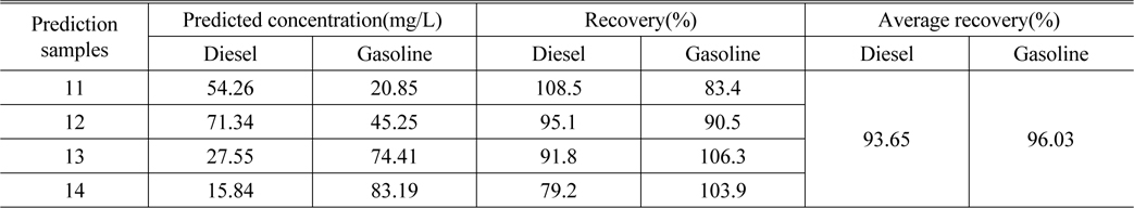
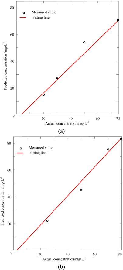
[FIG. 6.] The spectra of actual solution and SWATLD analyzed solution. (a) Fluorescence excitation spectra. “OOOO” : the actual spectrum of gasoline; “ΔΔΔΔ” : the actual spectrum of diesel; Factor 1 and factor 2: the components obtained by SWATLD algorithm. (b) Fluorescence emission spectra. “OOOO” : the actual spectrum of gasoline; “ΔΔΔΔ” : the actual spectrum of diesel; Factor 1 and factor 2: the components obtained by SWATLD algorithm.

Table 3 lists the actual concentration of diesel and gasoline in the samples #11 ~ #14, the prediction concentration obtained by SWATLD and the recovery rate. Figure 7 shows the least square fitting lines between the actual concentration of the samples #11 ~ #14 and the prediction concentration obtained by SWATLD. The correlation coefficients are 0.9845(diesel), and 0.9926(gasoline). It quantitatively shows that SWATLD has high resolution on the oil mixture.

[TABLE 3.] The predicted concentration and recovery of diesel and gasoline obtained by SWATLD

The predicted concentration and recovery of diesel and gasoline obtained by SWATLD

[FIG. 7.] The fitting lines between actual concentration and predicted concentration of diesel and gasoline. (a) R2 =0.9835, (b) R2 =0.9622.

   3.4. SWATLD for Mixed Solution of Diesel, Gasoline and Kerosene

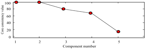
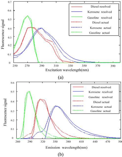
Scan the calibration samples #6 ~ #10 and prediction samples #15 ~ #18 to get the 3-dimensional data array , with the size of 9×37×21. Use the SWATLD algorithm to decompose . First, use the core consistent diagnosis method to estimate the number of components, as shown in Fig. 8. There is less difference in the core-consistency of 3 components and 4 components. As the SWATLD algorithm is not sensitive to component number, there is no need to estimate the component number accurately. We just need to make the component number greater than or equal to the actual component number to obtain the ideal results. Attempt to make the component number 3, and research the resolution of SWATLD on mixed oil. The excitation and emission spectra are shown in Fig. 9. The “diesel resolved”, “kerosene resolved” and “gasoline resolved” respectively represent the spectra of diesel, kerosene and gasoline obtained by the SWATLD algorithm. The “diesel actual”, “kerosene actual” and “gasoline actual” respectively represent the spectrum of actual diesel, kerosene and gasoline. We can conclude that the SWATLD algorithm has high resolution on 3 components oil mixture.

[FIG. 8.] Core consistency value of .

[FIG. 9.] The spectra of actual solution and SWATLD analyzed solution. (a) Fluorescence excitation spectra. The full lines represent the spectra of 3 components obtained by SWATLD algorithm; the imaginary lines represent the spectra of diesel, kerosene and gasoline respectively. (b) Fluorescence emission spectra. The full lines represent the spectra of 3 components obtained by SWATLD algorithm; the imaginary lines represent the spectra of diesel, kerosene and gasoline respectively.

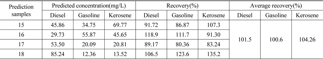
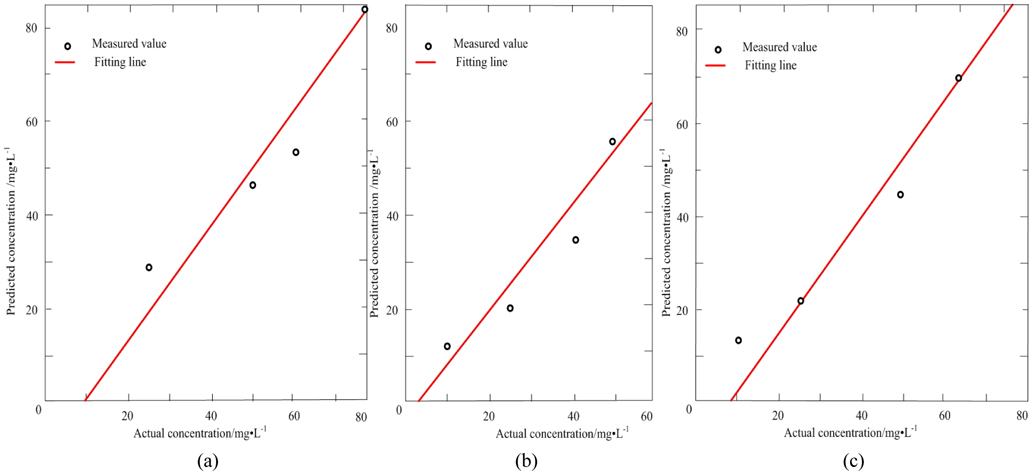
Table 4 lists the actual concentration of diesel, gasoline and kerosene in the samples #15 ~ #18, the prediction concentration obtained by SWATLD and the recovery rate. Figure 10 shows the least square fitting lines between the actual concentration and the prediction concentration obtained by SWATLD. The correlation coefficients are 0.9034(diesel), 0.9252(gasoline), 0.9643(kerosene). It is shown that SWATLD has high resolution on three or more kinds mixed oil.

[TABLE 4.] The predicted concentration and recovery of diesel, gasoline and kerosene obtained by SWATLD

The predicted concentration and recovery of diesel, gasoline and kerosene obtained by SWATLD

[FIG. 10.] The fitting lines between actual concentration and predicted concentration for diesel, gasoline and kerosene. (a) Diesel：R2=0.9536, (b) Gasoline：R2=0.9107, (c) Kerosene : R2=0.9646.

IV. CONCLUSIONS

Aimed at the problem of oil pollutants that are not easy to distinguish, a second order correction method was put forward. As the SWATLD algorithm is insensitive to factor numbers, there is no need to estimate the component number accurately. We just need to make the component number greater than or equal to the actual component numbers to obtain the ideal results. First, the diesel, gasoline and kerosene mixed solution was made up as calibration samples and prediction samples. Second, the FLS920 fluorescence spectrometer was used to measure the three-dimensional fluorescence spectra of the samples. The mixed solution spectra overlapped seriously, and it was difficult to distinguish each specific oil. And then the SWATLD algorithm was adopted to decompose the mixed oil. The decomposed spectra had high similarity with the measured spectra of each kind of oil. In addition, the concentration recovery rate was high. The experimental results show that the SWATLD algorithm has good effect on the separation of oil mixtures with overlapped spectra.

NOMENCLATURE

three-dimensional data matrix residual matrix A, B, C two-dimensional loading matrix xijk the ijkth element of aif, bif, ckf the ifth, jfth and kfth elements of loading matrix A, B, C eijk the ijkth element of the three-dimensional residual matrix σ the sum of squared residuals F the component number

참고문헌

1. Cohen M. A. (2013) “Water pollution from oil spills,” [Encyclopedia of Energy, Natural Resource, and Environmental Economics] Vol.3 P.121-126
2. Peiris R. H., Jaklewicz M., Budman H. (2013) “Assessing the role of feed water constituents in irreversible membrane fouling of pilot-scale ultrafiltration drinking water treatment systems,” [Water Res.] Vol.47 P.3364-3374
3. Insausti M., Fernandez Band B. S. (2015) “Single excitationemission fluorescence spectrum (EEF) for determination of cetane improver in diesel fuel,” [Spectrochimica Acta Part A: Molecular and Biomolecular Spectroscopy] Vol.140 P.416-420
4. Choi J. R., Kim K., Kim D. (2012) “In situ fluorescence optical detection using a Digital Micromirror Device (DMD) for 3D cell-based assays,” [J. Opt. Soc. Korea] Vol.16 P.42-46
5. Lee J., Pack C. G., Kim S. Y., Kim S. W. (2014) “Diffusion coefficients of CdSe/CdS quantum rods in water measured using polarized fluorescence correlation spectroscopy,” [J. Opt. Soc. Korea] Vol.18 P.598-604
6. Patra D. (2008) “Distinguishing motor oils at higher concentration range by evaluating total fluorescence quantum yield as a novel sensing tool,” [Sens. Actuators B: Chemical] Vol.129 P.632-638
7. Kavanagh R. J., Burnison K. B., Frank R. A. (2009) “Detecting oil sands process-affected waters in the Alberta oil sands region using synchronous fluorescence spectroscopy,” [Chemosphere] Vol.76 P.7
8. Fernandez M., Clavijo S., Forteza R., Cerda V. (2015) “Determination of polycyclic aromatic hydrocarbons using lab on valve dispersive liquid-liquid microextraction coupled to high performance chromatography,” [Talanta] Vol.138 P.190-195
9. Gao M., Wang H., Ma M. (2015) “Optimization of a phase separation based magnetic-stirring salt-induced liquid-liquid microextraction method for determination of fluoroquinolones in food,” [Food Chem.] Vol.175 P.181-188
10. Suranova M., Semanova J., Sklarsova B. (2015) “Application of accelerated solvent extraction for simultaneous isolation and pre-cleaning up procedure during determination of polycyclic aromatic hydrocarbons in smoked meat products,” [Food Anal. Method] Vol.8 P.1014-1020
11. Ferey L., Delaunay N. (2015) “Capillary and microchip electrophoretic analysis of polycyclic aromatic hydrocarbons,” [Anal. Bioanal. Chem.] Vol.407 P.2727-2747
12. Kalwa M., Quinaia S. P., Pletsch A. L., Torres Y. R., Finger D. (2014) “Polycyclic aromatic hydrocarbons in surface sediments of Binacional Itaipu Lake, Brazil: characteristics, sources and toxicity evaluation,” [Env. Earth Sci.] Vol.72 P.4473-4481
13. Ma Y., Cai C. Q., Yang H. M., Luo L., Chen X. M. (2014) “The amplified resonance light scattering signal detection of DNA hybridization using polycyclic aromatic hydrocarbons as a probe,” [Spectrosc. Lett.] Vol.47 P.184-191
14. Liaud C., Dintzer T., Tschamber V., Trouve G., Le C. S. (2014) “Particle-bound PAHs quantification using a 3-stages cascade impactor in French indoor environments,” [Env. Pollut.] Vol.195 P.64-72
15. Smolinski A., Kuna-Gwozdziewicz P., Laczny M. J., Bak A. (2015) “Study of the polycyclic aromatic hydrocarbons content in gas released from burning mine waste dump,” [Acta Chromatographia] Vol.27 P.239-254
16. Chen Z. K., Wang Y., Wang F. B., Wang Y. T., Zhou Y. (2014) “Excitation-emission matrix spectroscopy and parallel factor analysis for micro-content petroleum pollutant,” [Spectrosc. Spect. Anal.] Vol.34 P.2561-2567
17. Zhu B. Q., Pennell S. A., Ryan D. K. (2014) “Characterizing the interaction between uranyl ion and soil fulvic acid using parallel factor analysis and a two-site fluorescence quenching model,” [Microchem. J.] Vol.115 P.51-57
18. Parastar H., Akvan N. (2014) “Multivariate curve resolution based chromatographic peak alignment combined with parallel factor analysis to exploit second-order advantage in complex chromatographic measurements,” [Anal. Chim. Acta] Vol.816 P.18-27
19. Li L. J., Du S. X. (2012) “The three-dimensional fluorescence spectrometric detection of mycotoxin based on parallel factor analysis,” [Chin. J. Anal. Chem.] Vol.31 P.40-43
20. Zhang S. R., Wu H. L., Yu R. Q. (2015) “A study on the differential strategy of some iterative trilinear decomposition algorithms: PARAFAC-ALS, ATLD, SWATLD, and APTLD,” [J. Chemometr.] Vol.29 P.179-191
21. Li Y., Wu H. L., Qing X. D. (2013) “A novel method to estimate the chemical rank of three-way data for second-order calibration,” [Chemometr. Intell. Lab. Syst.] Vol.127 P.177-184
22. Yang L., Liu D. L., Wei Y. J. (2015) “Determination of Osthole in Cnidii Fructus and human plasma using excitation-emission matrix fluorescence with the aid of second-order calibration methods,” [Chin. J. Anal. Chem.] Vol.34 P.22-26
23. Hu L. Q., Yin C. L., Du Y. H., Zeng Z. P. (2012) “Simultaneous and direct determination of Vancomycin and Cephalexin in human plasma by using HPLC-DAD coupled with second-order calibration algorithms,” [J. Anal. Method. Chem.] Vol.2012 P.256963
24. Zhang J., Wang Z. J., Zhu S. R., Meng X. M. (2013) “Determination of sulfonamides in synthetic samples and pharmaceutical tablets using HPLC-DAD combined with SWATLD algorithm,” [Information Technology Applications in Industry] Vol.263 P.2117-2121
25. Bro R. (1998) “Multi-way analysis in the food industry, models, algorithms, and applications,” Ph. D. Thesis P.110-121
26. Ocana J. A., Barragan F. J., Callejon M. (2005) “Spectrofluorimetric and micelle-enhanced spectrofluorimetric determination of gatifloxacin in human urine and serum,” [J. Pharmaceut. Biomed. Anal.] Vol.37 P.327-332
27. Manzoori J. L., Amjadi M. (2003) “Spectrofluorimetric and micelle-enhanced spectrofluorimetric methods for the determination of gemfibrozil in pharmaceutical preparations,” [J. Pharmaceut. Biomed. Anal.] Vol.31 P.507-513

OAK XML 통계

이미지 / 테이블

[ FIG. 1. ] The decomposition diagram of PARAFAC model.
[ ]
[ ]
[ ]
[ ]
[ ]
[ ]
[ ]
[ ]
[ ]
[ FIG. 2. ] Process flow chart of SWATLD.
[ TABLE 1. ] The concentration of SDS micellar solution and the fluorescence intensity of kerosene SDS micellar solution
[ TABLE 2. ] The oil concentration in each sample (mg/L)
[ FIG. 3. ] 3-D fluoresence spectra of three standard samples. (a) 3-D fluoresence spectrum of diesel standard sample. Concentration: 10 mg/L; Width between excitation and emission slit: 1.11 mm; Excitation and emission step length: 5 nm; (b) 3-D fluoresence spectrum of gasoline standard sample. Concentration: 50 mg/L; Width between excitation and emission slit: 1.11 mm; Excitation and emission step length: 5 nm.; (c) 3-D fluoresence spectrum of kerosene standard sample. Concentration: 10 mg/L; Width between excitation and emission slit: 1.11 mm; Excitation and emission step length: 5 nm.
[ FIG. 4. ] 3-D fluoresence spectra of mixed samples. (a) 3-D fluoresence spectrum of a mixed solution of diesel and gasoline. Concentration of diesel and gasoline is 10 mg/L and 10 mg/L, respectively. Width between excitation and emission slit: 1.11 mm; Excitation and emission step length: 5 nm.; (b) 3-D fluoresence spectrum of a mixed solution of diesel, gasoline. and kerosene. Concentration of diesel, gasoline and kerosene is 10 mg/L, 10 mg/L and 10 mg/L respectively. Width between excitation and emission slit: 1.11 mm; Excitation and emission step length: 5 nm.
[ FIG. 5. ] Core consistency value of .
[ FIG. 6. ] The spectra of actual solution and SWATLD analyzed solution. (a) Fluorescence excitation spectra. “OOOO” : the actual spectrum of gasoline; “ΔΔΔΔ” : the actual spectrum of diesel; Factor 1 and factor 2: the components obtained by SWATLD algorithm. (b) Fluorescence emission spectra. “OOOO” : the actual spectrum of gasoline; “ΔΔΔΔ” : the actual spectrum of diesel; Factor 1 and factor 2: the components obtained by SWATLD algorithm.
[ TABLE 3. ] The predicted concentration and recovery of diesel and gasoline obtained by SWATLD
[ FIG. 7. ] The fitting lines between actual concentration and predicted concentration of diesel and gasoline. (a) R2 =0.9835, (b) R2 =0.9622.
[ FIG. 8. ] Core consistency value of .
[ FIG. 9. ] The spectra of actual solution and SWATLD analyzed solution. (a) Fluorescence excitation spectra. The full lines represent the spectra of 3 components obtained by SWATLD algorithm; the imaginary lines represent the spectra of diesel, kerosene and gasoline respectively. (b) Fluorescence emission spectra. The full lines represent the spectra of 3 components obtained by SWATLD algorithm; the imaginary lines represent the spectra of diesel, kerosene and gasoline respectively.
[ TABLE 4. ] The predicted concentration and recovery of diesel, gasoline and kerosene obtained by SWATLD
[ FIG. 10. ] The fitting lines between actual concentration and predicted concentration for diesel, gasoline and kerosene. (a) Diesel：R2=0.9536, (b) Gasoline：R2=0.9107, (c) Kerosene : R2=0.9646.