Each particular joint has the range of motion displayed by an angle [1]. Measurement on the motion of human joints is very important in screening of degenerative brain diseases such as Alzheimer’s disease, dementia and Parkinson’s disease, and the symptom of gait disability is presented in patients suffering from such diseases [2-4]. The symptom of gait disability is caused by limited range of motion, and it signifies the joint with reduced capacity for movement. Limited range of motion is caused not only by gait disability but also by mechanical problems due to certain joint injury or by diseases such as osteoarthritis and rheumatoid arthritis [5, 6].
Pain, swelling, and stiffness related to arthritis may limit the range of motion and damage function and capacity to lead daily lives. Physical therapy and rehabilitation treatment can be of great assistance in improving the function of a joint by focusing on range of motion exercise [7, 8]. The objective of this exercise is not only to reduce the pain, swelling, and stiffness but also to smoothly increase the range of motion.
Currently, there is an increase in market demand for quick measurement of change in motion of human joints. Since there are various medical fields which benefit from angular motion measurement, the necessity for monitoring of human joint movement is increasing. There are various medical applications, and the most general application is in physical and rehabilitation treatments [9-11]. The monitoring of human joint movement not only provides benefit in the field of medicine but also in sports [12].
There are goniometers and electro-goniometers as devices to be used for such a purpose. However, previous goniometers have limitations in abrasion of electric moving parts, durability, and size. An optical sensor has the strength in outstanding durability without abrasion in its moving part and it can be manufactured in small size with the use of optical fiber. Thus, studies on a goniometer that can measure angle with the use of light were conducted in order to avoid the weaknesses of previous goniometers. Most of optical fiber goniometers were based on the bending loss of light signal [2, 8, 13]. Recently, joint angle measurements were performed with modified fiber tips [14]. However, the measuring ranges of optical fiber goniometers were limited and the whole range of angular motion could not be detected.
In this study, the optical sensor is composed of a light emission unit which emits the light and a light reception unit that receives the intensity of radiation. The light emission unit is combined of a red LED and an optical fiber. The reason why optical fiber is utilized is that it is thin and flexible. Also, since total reflection occurs inside, there is no loss of light, thus it can be effectively used as an optical sensor. For the reception unit, three photodiodes were arranged to increase the measuring range of angular motion. The optical signal detection range was widened with the use of multiple photodiodes and the result will be useful for designing an effective angular sensor with low cost and small size.
2.1. Shape of Beam Output Based on Tip Angle of Optical fiber
Previous study showed that a certain tip angle caused the increased detection range of the joint angle measurement with a single photodiode in the light reception unit [14]. The redirected beam caused an asymmetric beam pattern and broadened the angle measuring range. Thus, we need to confirm the effect of fiber tip angle on measuring range of the joint angle.
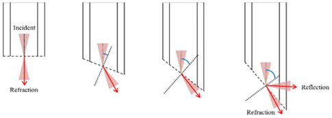
Figure 1 shows the change in beam output based on change in tip angle of the optical fiber. When the incidence angle is entered with another medium with different refractive index, refractive light is determined by Snell’s law. With small incidence angle, most of the light is refracted and one beam direction is presented. However, with the increase in incidence angle followed by increase in tip angle of the optical fiber, some of the refracted light is reduced and there is an increase in reflected light. Therefore, two beam directions are presented from a particular angle.
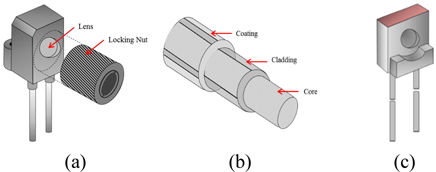
Figure 2 shows the light source of the light emission unit and the photodiode of the light receiving unit that are used in the experiment. Figure 2(a) shows the light source IF-E96 (Plastic Fiber Optics Red LED), and it presents a red visible ray with peak wavelength of about 660 nm. Also, it can be used to hold the optical fiber and it has the strength of an effective micro-lens for efficient optical coupling, low-cost, and high-speed. Figure 2(b) shows optical fiber (BFL48-1000, Thorlabs) with 0.48 of NA (Numerical Aperture), core with diameter of 1,000 um, and cladding with diameter of 1,035 um thus total diameter is very thin presenting 1,400 um. Figure 2(c) shows the photodiode (ST-23G, Kodenshi) used as the light-receiving unit and it presents spectral sensitivity of 500 ~ 1,050 nm and half angle of ± 30°. Spectral sensitivity of the photodiode used as a light-receiving unit can accommodate peak wavelength of light-emission unit thus it is appropriate to be used in the experiment.
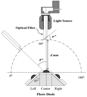
Figure 3 shows the experimental setup used in this study. Left and right photodiode sensors are attached to a center sensor at 45°, and the center sensor is placed to rotate about a central axis after installing it on a stage which is adjustable in X and Y directions. Optical fiber is fixed to an angle indicated rotation stage which enables rotation after connecting it to the light source. The rotation angle when the optical fiber and center sensor are on the straight line is referred to as θ = 90°. At that time, the distance between center sensor and optical fiber was defined as d. Variables used in the experiment include the distance between center sensor and optical fiber (d = 13 mm ~ 15 mm), tip angle of optical fiber (φ = 0° ~ 40°), and rotation angle of optical fiber (θ = 0° ~ 180°). Analysis of the joint angle was conducted through an algorithm by transmitting the light that comes out from the light source without a loss through the optical fiber, real-time measurement of change in optical output signal (V) from three sensors through LabVIEW and MATLAB programs.
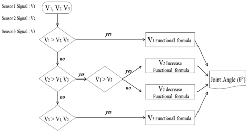
In order to measure joint angle with the change in intensity of radiation that is received from the three sensors, a functional formula was acquired with inverse mathematical modeling regarding the three output signals with the use of MATLAB. Then, the angle was detected through an algorithm as illustrated in Fig. 4. By comparing the values for the three sensors, the joint angle was detected by subjecting the voltage value to an inverse mathematical modeling functional formula that corresponds to the signal that has the highest peak value.
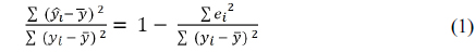
Since the inverse mathematical model can be used in a domain which presents the tendency of continuous increase or decrease [15], the modeling was conducted with division into increase and decrease domain for each sensor. In the inverse equation, x refers to the voltage value and y refers to angle. In other words, it was made so that the output voltage value can be converted into joint angle with the inverse mathematical model and angle could be detected with only minute change in voltage value. Also, the coefficient of determination (R2), an index to measure the adequacy of the regression equation acquired through modeling with original data, could be acquired. The coefficient of determination has a value between 0 and 1 and a value close to 1 signifies that all data is close to the associated functional formula. It can be acquired with Eq. (1).

3.1. Shape of Beam Output Based on Distance Between Sensor and Optical Fiber
Figure 5 shows the shape of beam output based on distance (d) between center sensor and optical fiber (φ = 0°). Figure 5(a) shows that resolution is low with left and right sensor outputs at d = 10 mm since the distance between the light-receiving unit and the optical fiber is close. Figure 5(b) shows that output is stable and there is an increase in peak value of the left and right sensors, and a decrease in peak value of the center sensor compared to Fig. 5(a). However, when d = 15 mm as illustrated in Fig. 5(c), there is a decrease in overall peak value and the output of the center sensor becomes unstable. Therefore, the distance of d = 13 mm between the center sensor and the optical fiber is most satisfactory with high peak values of left and right sensors and enough output of the center sensor.
3.2. Shape of Beam Output for Each Sensor
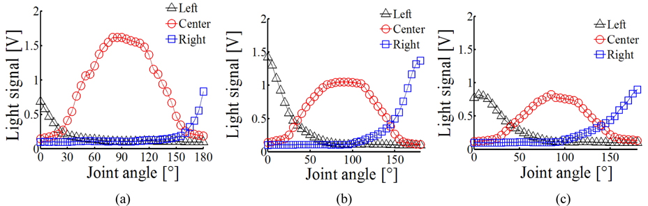
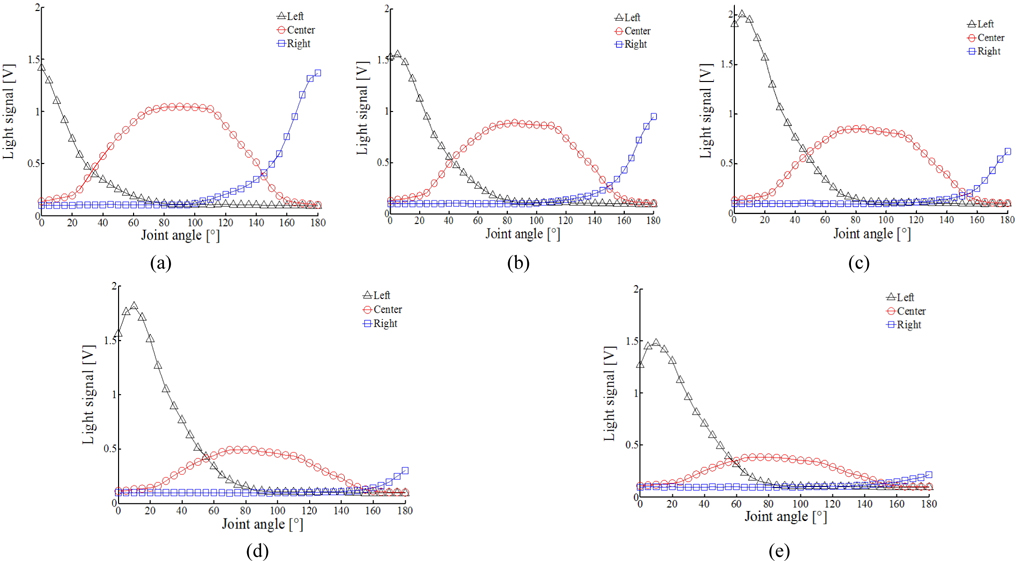
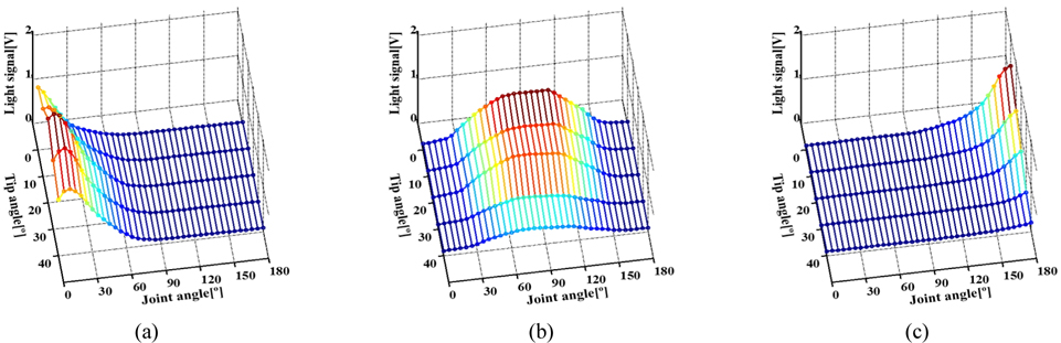
Figure 6 shows the beam output signal based on change in tip angle (φ) and joint angle (θ) when d = 13 mm. As illustrated in Figure 6(a), the peak value for the left sensor first increases then decreases with the increase in tip angle of the optical fiber. It is due to the fact that there is a decrease in intensity of radiation received with division into two beam directions followed by the increase in tip angle of optical fiber as illustrated in Fig. 1. Peak values for center and right sensors, as shown in Figs. 6(b) and 6(c), decrease with the increase in tip angle of the optical fiber and measurement range of joint angle narrowed down.
3.3. Shape of Beam Output Based on Tip Angle of Optical Fiber
Figure 7 shows the shape of beam output based on tip angle of the optical fiber. In the left sensor, as shown in Fig. 7(a), the output from flat fiber tip (0°) shows a monotonically decreasing pattern with relatively high light intensity. For the cases of angled tips, as shown in Figs. 7(b) ~ (e), the outputs show initially increasing and then decreasing patterns which are not monotonic patterns. To obtain joint angle values directly from output light signals in real time, inverse functions are required. The inverse model is possible when the functions show monotonic patterns of increase or decrease. Thus, the data should be divided into two sections (increasing and decreasing sections) for the cases of angled tips. However, the increasing sections of angled tips do not have enough data points for curve fitting.
For the outputs from the center sensor (Fig. 7), all outputs from both flat and angled tips do not show monotonic patterns, but they can possibly be divided into two monotonic sections for inverse modeling with enough data points. For the outputs from the right sensor, all outputs show monotonic patterns and the output from the flat tip shows the highest intensity over the outputs from the angled tips. There is a lowering of sensitivity with the decrease in intensity of radiation in the right sensor followed by the increase in tip angle of the optical fiber. Therefore, it is determined that it is optimal when the tip angle of the optical fiber is φ = 0° for the whole measurement range of θ = 0° ~ 180°. Alternatively, the tip angle of 20° with the highest light intensity (Fig. 7(c)) can be used for a monotonic section in a small range (5 ~ 80°) of joint angle measurement.
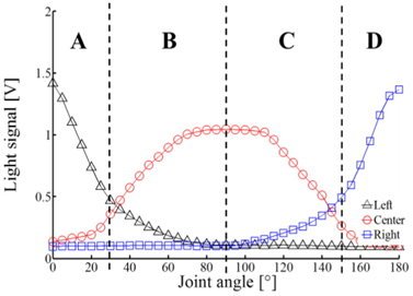
Since the inverse modeling can be applied to monotonically increasing or monotonically decreasing regions, the angular regions were divided into four sections, as shown in Fig. 8, for inverse mathematical modeling when d = 13 mm and φ = 0° which is most appropriate to detect the joint angle. In Section A, the left sensor signal showed high resolution; in Sections B and C, the center sensor signal showed high resolution; in Section D, the right sensor showed high resolution.
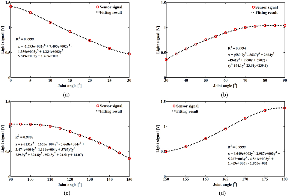
Inverse functions are required to obtain directly joint angle values from light signal outputs. Polynomial, exponential, and power functions were tested for the possibility of practical use. With high R2 and small RMSEs, the inverse 5th order equation showed the best fit to data. The 5th order equation was selected for the practical purpose of obtaining joint angle values with LabVIEW display in real time.
Figure 9 shows the inverse modeling results in each section with 5th order polynomial equations. The coefficient of determination (R2) and p-value of each section are (a) R2 = 0.9999, p < 0.01, (b) R2 = 0.9994, p < 0.01, (c) R2 = 0.9988, p < 0.01, and (d) R2 = 0.9999, p < 0.01. This implies that the equations obtained are correlated well with measured data.
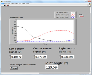
Figure 10 shows the example of LabVIEW display for angle detection. In regards to angle detection, it shall be detected with the use of a functional formula of the left sensor since the signal of the left sensor is large from 0° to 30°. In the case of 30° ~ 150°, the angle is acquired with the use of a functional formula for the center sensor since the signal of the center sensor is strong. In the case of 150° ~ 180°, the angle is acquired by using functional formula of the right sensor as a signal of the right sensor being strong. The value of joint angle can be detected with curve fitting and the algorithm described in Figs. 4 and 9.
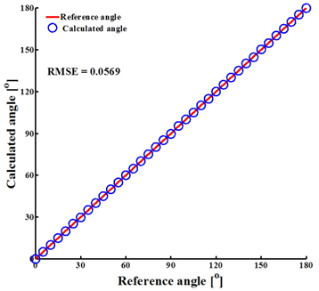
Figure 11 shows the relationship between the reference joint angle and the calculated angle from the proposed sensor with inverse models and LabVIEW display. The calculated angles are correlated well with the reference joint angle. R2 is 0.9999 with
Previous angle measurement methods have weaknesses in accuracy, abrasion, durability, and size. In this study, new measurement technology using light was proposed so that it could avoid the weaknesses of previous angle measurement methods. For this achievement, relatively inexpensive, small, and light optical fiber without abrasion by electrical resistance and photodiodes with high sensitivity were used so that specific angles could be detected precisely.
In order to broaden the range of measurement, three photodiodes were used with the change in beam profile from the optical fiber. It was possible to measure the joint angle with the intensity of radiation using inverse mathematical modeling and an algorithm. In future studies, research on the increase in the number of various sensors, change in sensor attaching angle, and other factors will be conducted in order to come up with the program which can measure the angle in real-time to enable more convenient application for its users.