Against the backdrop of increasing uncertainly in the recent economic conditions, a method of evaluating economic rigidity and safety of investment alternatives is of practical importance. Economic evaluation of rigidity and safety was developed in the area of engineering economy (Senju
This paper examines a simple model of investment alternatives over multiple periods, composed of unit variable cost and fixed cost over each period. For the product, unit sales price and sales volume over each period is estimated. The paper analyzes a case of uncertainty in which one of the values for these four factors under consideration move worse toward the direction of decreasing profit. The paper first identifies the breakeven point for each of the four factors, and shows the values of these breakeven points on the normalized TC-UC domain, whose horizontal axis represents total cost and vertical axis, unit-cost. Then the paper discusses an area on the normalized TC-UC domain where alternatives safer for all of the four factors are plotted. Thus, a practical and visual method of rigidity analysis for investment alternatives is formulated and proposed.
This section summarizes assumptions and notations of the model for analysis.
1) The planning horizon covers n periods. For the j-th period, as sales conditions, unit sales price and sales volume for the product under consideration are esti-mated and denoted by pj and Qj, j = 1, 2, …, n, respectively.
2) As production conditions, cost structure for producing the product is given by unit variable cost vj and fixed cost Fj over the j-th period, j = 1, 2, …, n. The sales volume is assumed to be equivalent to production volume in each period.
3) Capital cost, which is common over the entire planning horizon, is given by interest rate i.
4) Product is designated by A, B, C, … and represented by subscript when necessary.
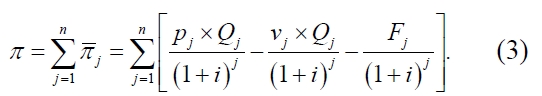
Based on these assumptions, the profit for the
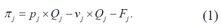
Its discounted present value considering capital cost is obtained by
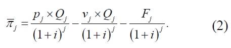
It follows that the total sum of profit over the entire planning horizon is represented by
This section analyzes breakeven points for each of the four factors, for the purpose of comparing rigidity against unexpected changes in each of the four factors under consideration.
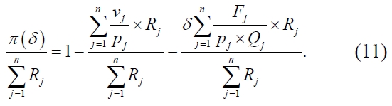
It should be noted that the value of total profit
Here, we denote the total sales for the
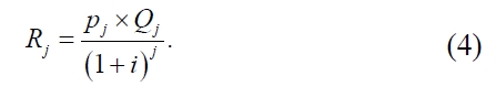
Then from statement (2),
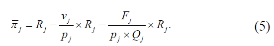
It follows,
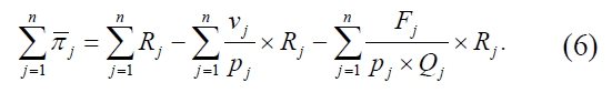
Therefore,
This paper investigates the following changes in each of the four factors, which is assumed to be independent of each other:
Decrease in unit sales price;
pj → α Pj, 0 < α < 1, j = 1, 2, …, n.
Decrease in sales volume;
Qj → βQj, 0 < β < 1, j = 1, 2, …, n.
Increase in unit variable cost;
νj → γνj, γ > 1, j = 1, 2, …, n.
Increase in fixed cost;
Fj → δFj, δ > 1, j = 1, 2, …, n.
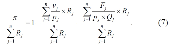
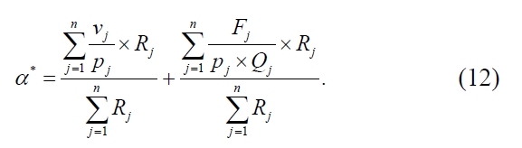
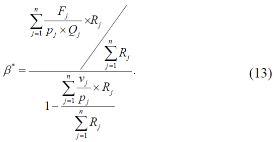
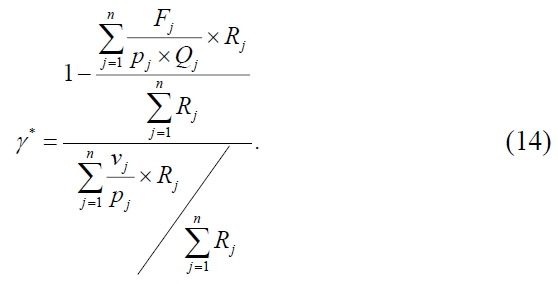
From statement (7), the following equations can be obtained.
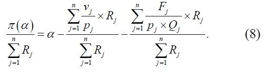
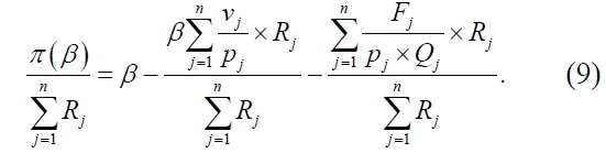
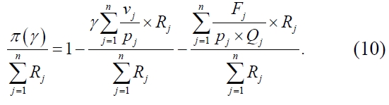
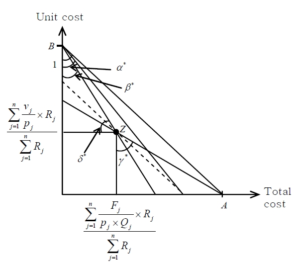
Then, the breakeven point for each factor, denoted by
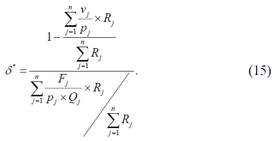
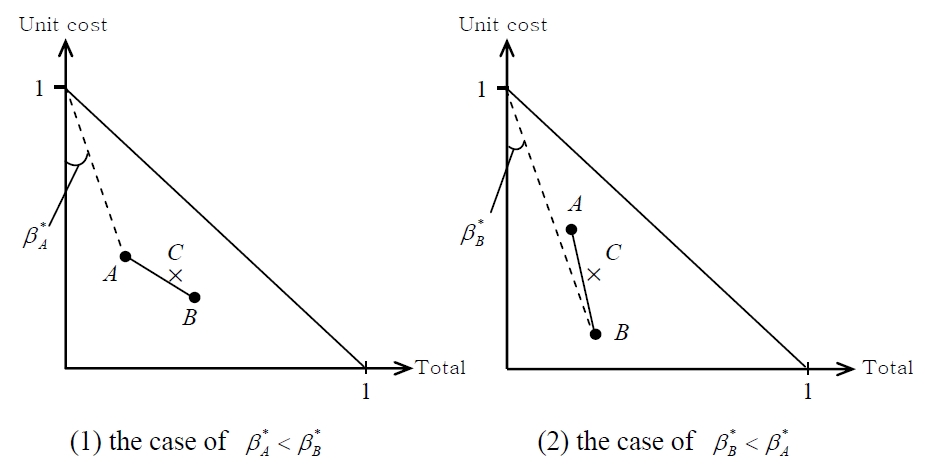
On the TC-UC domain whose axes are normalized to the scale of (1, 1), the values of these breakeven points can be represented as shown in Figure 1.
This section analyzes, on the normalized TC-UC domain, the area in which alternatives are safer against all the changes in values on the four factors. For simplicity plicity of description, the paper defines following notations:
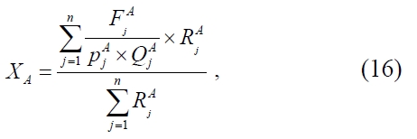
and
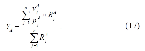
where subscript represents product identification.
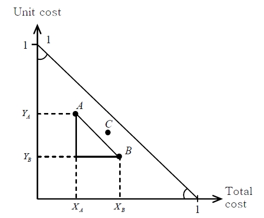
We assume two alternatives A and B, as illustrated in Figure 2, where

as shown in Figure 2, The plot C satisfies
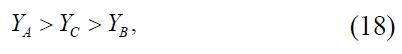
and
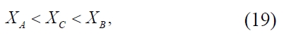
and
This implies that plot C is located up right against
resulting that line segments connecting A, C, B shapes concaveto down left.
Under these conditions, it is clear that either
Against decrease in sales volume, as shown in the case of
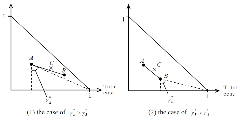
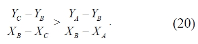
Against increase in unit variable cost, where
>
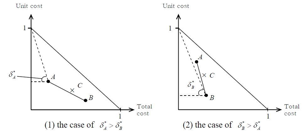
Lastly, against increase in fixed cost, two cases can be found as shown in Figure 5. Where of
As a result of the above discussion, a safer alternative than both A and B can never create concave to down left against line segment
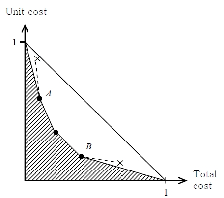
Therefore, a safer area for a given set of alternatives is the area down left to the convex line segments given by connecting adjacent plot of alternatives as described in Figure 6.
Further, for the convex line segments on the TCUC domain, we shall investigate upper end and right end, as described in Figure 6. Let denote plots A and B as in the figure. At the upper end, setting a scale verticallyon the verticalax is and turning it anti-clockwise centered on the point (0, 1), we can conclude that an alternative located in the upper right to the line segment connecting (0, 1) and plot A in Figure 6 is inferior in safety against changes in all of the four factors. In the same context, setting a scale horizontally on the horiontalax is and turning it clockwise centered on the point (1, 0) on the TC-UC domain, an alternative located in the upper to the line segment connecting (1, 0) and plot B on Figure 6 is also inferior in terms of safety against changes in the four factors.
Therefore, a safer area against changes in the four factors under consideration is represented as an area down left to the convexset of line segments as represented in Figure 6.
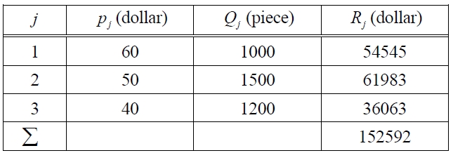
For simplicity, the paper takes a case of a single product. The paper assumes that the target life for the product is 3 years. For the sales conditions, the base case is given in Table 1. On the other hand, the base case of production is given in Table 2.
[Table 1.] Base Case on Sales Conditions.

Base Case on Sales Conditions.
At this point, we consider several alternative cases for each of sales case and production case as follows;
For sales:
Base case I): pj and Qj are given as in Table 1.
Scenario II): pj is increased to 120% in each year from the base case, and Qj is decreased to 80% in each year from the base case.
Scenario III): pj is increased to 150% in each year from the base case, and Qj is decreased to 60% in each year from the base case.
For production:
Base case a): vj and Fj are given as in Table 2.
Scenario b): vj is reduced to 85% in each year from the base case, while Fj is increased 150% in each year from the base case.
Scenario c): vj is reduced to 80% in each year from the base case, while Fj is increased to 200% in each year from the base case.
For the base case combination which is described as a-I,
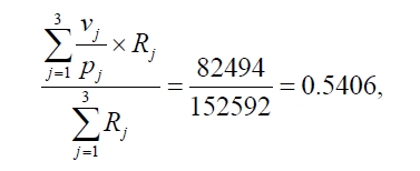
and
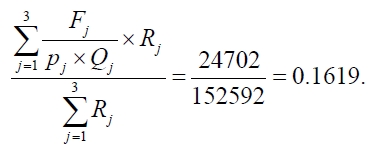
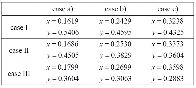
Similarly in the same manner, the x-y values of plots on the normalized TC-UC domain in each combination of sales case and production case are summarized in Table 3.
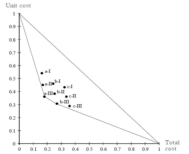
Then, we can plot all of nine combination cases on the normalized TC-UC domain, which is illustrated as in Figure 7. Clearly from this Figure, starting from plot (1,
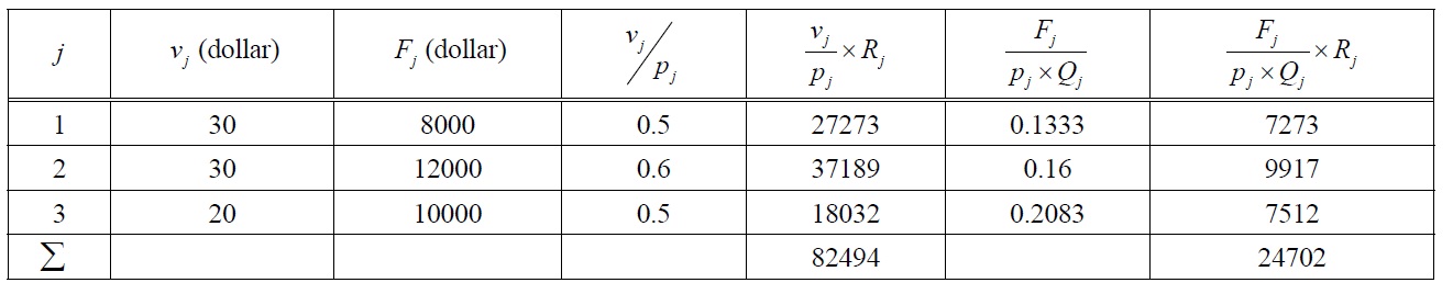
[Table 2.] Base Case on Production Conditions.

Base Case on Production Conditions.
0) and ending up at plot (0, 1), the convex line segments are organized by plots of a-III and b-III. It means that these two combinations are rigid against unexpected change in factors under consideration, but the other seven combinations can never be safer against changes in all factors under consideration. Thus, for this numerical example, applying the proposed procedure on the normalized TC-UC domain, we can point out production scenario C is disqualified in terms of economic rigidity against unexpected changes in factors, as well as sales scenarios I and II which are also disqualified. Thus, we can concentrate risk estimation on production scenario a and b, and sales scenario III, more specifically a-III and b-III. Thus, the proposed method can be a practical tool for eliminating disqualified alternatives in terms of risk and rigidity, and enable focusing on a limited number of alternatives for detailed risk and rigidity analysis. Thus,
[Table 3.] x-y Coordinates of Plots for Each Combination.

x-y Coordinates of Plots for Each Combination.
alternatives for detailed risk and rigidity analysis. Thus, the proposed method can support economic risk evaluation of investment alternatives.
1)The proposed method of rigidity analysis is valid for an arbitrary fluctuation of the four factors, i.e. unit sales price, sales volume, unit variable cost, and fixed cost, over the planning horizon. But for the sake of illustrating practical utilization, the numerical example is divided into sales conditions and production conditions.
This paper analyzed a problem of safety analysis for a set of alternatives over multiple periods. As a visual tool to represent a safer area, the paper proposed twodimensional domain named normalized TC-UC domain.
On the domain, breakeven points for each of the four factors, unit sales price, sales volume, unit variable cost, and fixed cost, are represented. Applying the result of breakeven point, the paper presented a safer area, against changes in the values of the relevant factors under consideration, on the normalized TC-UC domain. By plotting multiple alternatives on this domain, we can evaluate rigidity of given investment alternatives under uncertainties. Thus, the proposed TC-UC domain can work as a practical tool for economic rigidity evaluation.
The model can be extended to deal with such cases as simultaneous and dependent changes of relevant factors, distinction of production volume and demand quantity, and varying change ratios over the multiple planning periods. Analysis of these cases is left as an area for future research.