Over the past few decades, underwater acoustic communication (UWAC) has been studied by many researchers. Recently, these studies have focused on areas such as pollution monitoring for environmental systems, remote-control operations in the marine oil industry, the collection of scientific data from the deep sea, and the localization of submarines. In many commercial and military applications, the need for real-time communication with submarines and deep-sea unmanned systems has increased. The main restrictions when transmitting signals underwater are the characteristics of the sea, which fluctuate rapidly in a complex manner. The channel environment for UWAC in shallow water affects the propagation velocity of signals depending on the depth of the water, the distribution of the water temperature, and the salt concentration.
It is difficult to communicate in underwater environments for many reasons, such as multipath effects, Doppler effects, noise, and attenuation. These lead to errors in the communication performance and maximum propagation distance that can be realized. In particular, the multipath propagation phenomenon appears because of wave reflection in the sea level and the ocean floor. For these reasons, UWAC has more limitations compared to terrestrial radio communications. Further, with UWAC, it is difficult to increase the communication capacity, which depends on the signal bandwidth, because UWAC uses a very low carrier frequency in the ultrasonic band compared with terrestrial radio communications owing to the media channel characteristics. Nevertheless, the underwater channel is used in UWAC, and it is commonly realized using sound waves or acoustic communications.
Direct-sequence code division multiple access (DS-CDMA) [1, 2], orthogonal frequency-division multiplexing (OFDM) [1, 3-5], and multi-input multi-output (MIMO) [1, 6], modulation and error correction [7], and others [8-11] techniques that can transmit high-speed data are commonly employed in UWAC.
In this study, we calculate the propagation distance that can be realized using the DS-CDMA technique with directsequence spread spectrum (DSSS) in underwater communication systems, considering only the attenuation and noise as limiting factors. We also compare the estimated and calculated distances obtained for different scenarios.
2. Attenuation and Noise Condition for Underwater Acoustic Transmission of DS-CDMA
A unique property of acoustic channels is the dependence of the path loss on the signal frequency. This dependence exists because of absorption, i.e., the conversion of acoustic energy into heat. In addition to absorption loss, the signal experiences a spreading loss that increases with distance. The overall path loss is given by Eq. (1).
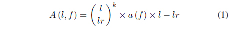
where ƒ is the signal frequency and
In an acoustic channel, the noise comprises ambient noise and site-specific noise. The ambient noise, which is always present, may be modeled as Gaussian noise, but it is not white, and its power spectral density (PSD) decays at approximately 18 dB/decade.
If we define a narrow band of frequencies of width Δƒ around some frequency ƒ, the signal-to-noise ratio (SNR) in this band can be expressed by Eq. (2).
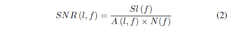
where
3. DS-CDMA Technique with Gaussian White Noise
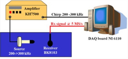
In this section, we present a case study that involves the application of only Gaussian white noise in a DS-CDMA receiver with DSSS. In order to perform the experiment in the case study, we organize an experimental device, as shown in Figure 1.
In Figure 1, we use as the source a transducer with a resonant frequency of 36 kHz, an operating depth of 50 m, and an operating temperature of 25℃.
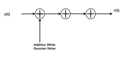
Figure 2 represents the block diagram that we employed when considering only additive white Gaussian noise (AWGN) during a review of real conditions in UWAC.
In our experiment, we estimate the distance as 50 m. To determine the time of flight (TOF), we first determine the speed of sound at a depth of 50 m (the operating depth of the transducer), and we can obtain an estimate of the TOF using the estimated distance.
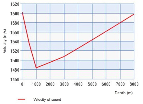
The velocity of sound in seawater varies with water pressure, temperature, and salinity, and it is calculated using the Del Grosso or UNESCO formula. The temperature of the seawater is assumed to be 4℃ at a depth of 1000 m, and 2℃ at a depth of 3000 m or more, as shown in Table 1.
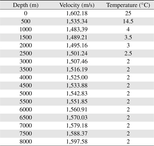
Velocity of sound
From Table 1, we obtain a graph of the velocity of sound as shown in Figure 3. We can obtain the corresponding velocity of sound at a certain depth. Now, we choose a channel depth of 50 m with a salinity of 34%. From Table 1 and Figure 1, we obtain the speed of sound as 1595.496 m/s. Therefore, we obtain the following TOF as Eq. (3) because we can calculate the distance using the formula: distance = speed × time. We perform the conversion using sample delay numbers, and we obtain a delay for 23,817 samples. Therefore, we can estimate the following values: sample delay = 23,800 samples, TOF = 0.62676 s, distance = 1000 m.
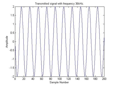
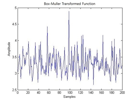
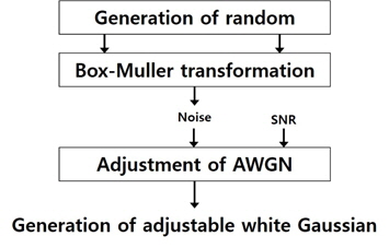
We consider the underwater operating conditions to determine the following communication parameters. The transmitting frequency, operating depth, operating temperature, and wind velocity are 36 kHz, 50 m, 25℃, and 0 m/s, respectively. We have to find the sound level that corresponds to these conditions. To do this, we use the PSD of the ambient noise. From the PSD data of the ambient noise, we found that for a frequency of 36 kHz and a wind velocity of 0 m/s, the sound level of ambient noise is 30 dB. Furthermore, we added ambient noise to the transmitted signal with a delay equaling 23,800 samples. We obtained the following calculated results. Figure 4 shows the transmitted signal with a frequency 36 kHz. To generate ambient noise of 30 dB, we first generate a random signal and then perform a Box-Muller transform. We add noise in order to vary the AWGN. Figure 5 shows the generation of the adjustable white Gaussian noise.
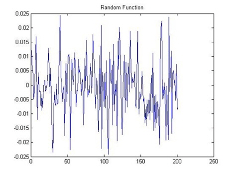
Figure 6 shows the generated random signal. To generate the Box-Muller transformed noise, we use the formula in Eq. (3).

We obtain the graph of signal X, as shown in Figure 7.
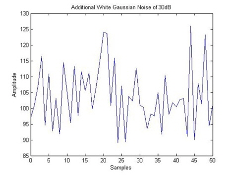
The next step includes the adjustment of the previously generated noise after the Box-Muller transformation into an AWGN with a sound level equal to 30 dB.
Mathematically, we represent the AWGN using Eq. (4).

Using Eq. (4), we obtain Figure 8 for an AWGN of 30 dB.
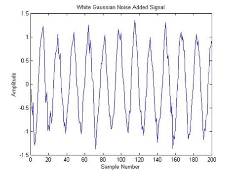
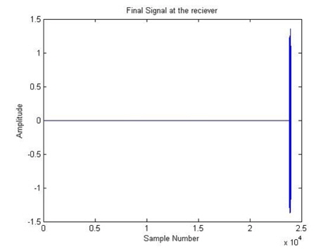
We need to modulate the signal and calculate the TOF. To do this, we have to add the white Gaussian noise signal to the transmitted signal, including the sample delay of 23,800 samples, in order to modulate the final received signal. Then, we take the cross correlation of the final signal with the transmitted signal to calculate the TOF. Figure 9 shows that the AWGN signal is combined with the transmitted signal. The delay sample can be computed using MATLAB as a value of 23,778 samples. Figure 10 depicts the delay of 23,778 samples, which are the final signals at the receiver.
Finally, we can calculate the TOF using Eq. (5).

where the TOF is the time of flight, DS is the number of delay samples, and SF is the sample frequency.
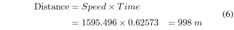
From Eq. (5), we obtain the TOF as 0.62573 s.
We also calculate the distance using Eq. (6).
In Table 2, we present a comparison of the estimated and calculated values for the TOF and distance.
[Table 2.] Comparison of estimated and calculated values for the time of flight and distance
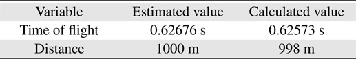
Comparison of estimated and calculated values for the time of flight and distance
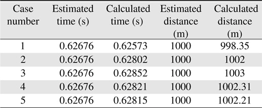
We also consider the following scenarios:
Case 2: shipping activity 0.5 and wind speed 0 m/s. (48 dB)Case 3: shipping activity 1 and wind speed 0 m/s. (48 dB)Case 4: shipping activity 0 and wind speed 10 m/s. (25 dB)Case 5: shipping activity 1 and wind speed 10 m/s. (25 dB)
We obtain the estimated time, estimated distance, and calculated distance for each case, and we present them in Table 3.
[Table 3.] Result for estimated time, estimated distance, and calculated distance for each case

Result for estimated time, estimated distance, and calculated distance for each case
In this study, we estimate and calculate the propagation distance for the DS-CDMA technique with DSSS in an underwater communication system, considering only the limitations due to the attenuation and noise. Based on our comparison of the estimated and calculated distances, we find that there is little difference between them in an underwater system. This implies that we can apply the proposed calculation method to determine the propagation distance in an underwater system for DS-CDMA communications, even though underwater systems are prone to attenuation and noise.